1 INTRODUCTION

Full waveform inversion (FWI) is used to reconstruct the subsurface model by minimizing the difference between the observed and synthetic data (Tarantola, 1984). Theoretically, FWI can potentially extract the maximum amount of information from seismic data by taking many factors into consideration, such as many media parameters, all kinds of wave propagation phenomena and all the seismic information. During the past decades, with the development of computational power, the better quality of seismic data and especially the successful application of reverse time migration, FWI has shown a great progress on both methodology study and application research.

However, the strong nonlinearity caused by the complex relationship between the seismic data and the media parameter (Jannane et al., 1989; Dong et al., 2013) is still the main difficulty for FWI (Virieux and Operto, 2009). Furthermore, the application of FWI to real data also has many challenges, such as the lack of long offset and low frequency contents, the unknown source wavelet, the poor initial model, the inaccurate wave propagation theory, the low S/N ratio and so on. All the difficulties aforementioned prevent FWI from being applied in practice. Hence, in seismology, FWI still cannot take the place of travel time or finite frequency tomography; while in seismic exploration, FWI cannot replace the traditional procedure of seismic data processing and interpretation. It is reasonable to deal with the low and high wave numbers of the subsurface model separately in the conventional seismic data processing and interpretation and it is a basic idea and strategy for us to handle the complex problem step by step. Considering about the theoretical difficulty and the complexity of the field seismic data, FWI, which is on the way of maturity, also should lower its status and face the reality. It means that it is not necessary for FWI to pursue exploiting all the information in the data during inversion, because the background model can be constructed and the strong nonlinearity can also be reduced by matching part of the information of the seismic data only. Admittedly, the inversion resolution would be reduced by this way, but it is better than the inaccurate high resolution model which can do nothing to improve the quality of migration image.

Based on the aforementioned concerns, we present a strategy of waveform inversion based on seismic data subset. In the following, we firstly present the basic idea of waveform inversion based on seismic data subset and give out the uniform gradient formula for different data subset. Finally, inversion tests with synthetic and field data are carried out to prove the correctness and effectiveness of such strategy.

2 METHODOLOGY 2.1 Basic Idea

The conventional FWI is performed in an attempt to obtain an earth model by reducing the discrepancy between the observed and synthetic data. The discrepancy is quantitatively defined by a misfit function under the least square principle as

(1)

Here, m stands for the model parameters, and h₁ is a function that measures the similarity between the synthetic and observed data. T is the time length of seismic records, U is the real number space where the wavefield u belongs. The media parameter m(x) ∈ M, and M is the model space. Apparently, h₁ is the mapping from the space of U × M to the space of R and J is the mapping from the model space M to the data space R.

The relationship between the data residual and model perturbation can be formulated as

(2)

where ∆d, K and ∆m are the data residual, Fr´echet derivative (kernel function), and the model perturbation vector, respectively.

If the relationship between data and model parameters is close to linearity, it is reasonable to use Eq.(2) to handle all the seismic data and the subsurface model parameters together. However, there are different components in the subsurface model and different contents or subsets in the seismic data. For example, there are low and high wavenumbers in the subsurface model, there are different types of seismic phases, such as refracted wave, reflected wave, surface wave, and there are different kinds of information in seismic data, such as travel time, amplitude, waveform, etc. The nonlinear relationship between different data subsets and model parameters are not the same (Dong et al., 2013). Different components of model exhibit on different seismic phases and different seismic information. For example, the perturbation of low wavenumber of the velocity model mainly corresponds to the travel time of reflected waves, while the high wavenumber to the amplitude. The first arrival time is mainly affected by the shallow velocity of the model while the reflected wave from the deep part of the model is affected by all the structures in the shallow, middle and deep part of the model. The complex relationship between different data subsets and model components reveals that different data subsets have different inversion ability. It reminds us that the details of their relationships should be analyzed carefully in order to effectively reduce the nonlinearity of FWI. Specifically, we should modify the Eq.(2) to Eq.(3),

(3)

where ∆d_i, ∆m_j and K_ij stand for the data subset residual, the perturbation model vector, and sub-kernel describing the relation of ∆d_i and ∆m_j, respectively.

By above analysis, we come to the conclusion that the perturbation for different components of the model is mainly dependent on the sub-kernel and data subset residual. So far, there are two ways to calculate the model perturbation: one is the adjoint-state method (Tarantola, 1984; Tromp et al., 2005; Plessix 2006) which back-projects the data residual along the kernel (wave path); the other is scattering integral method (Zhao et al., 2005; Chen et al., 2007; Liu et al., 2015) which explicitly calculates and stores the kernel, then solves the inversion matrix. The basic idea of our inversion strategy based on seismic data subsets is that, by analyzing the seismic data subset and its corresponding kernel, we can decide which part and which wavenumber of the subsurface model can be updated according to our requirement at different inversion stages.

The characteristics of the kernel and its calculation are two crucial points in finite-frequency tomography (Dahlen et al., 2000; Tromp et al., 2005; Liu et al., 2009), wave equation tomography (Woodward, 1992) and full waveform inversion (Tarantola, 1984; Pratt, 1998; Virieux and Operto, 2009). The information contained in each data subset is quite different from each other, and the kernel for different data subsets and components of the subsurface model is significantly different. Hence, different kernels should be used for different information of seismic data to decouple the low and high wavenumber components of the model (Chi et al., 2015). Refracted wave travel time is sensitive to the shallow and middle part of the background velocity. If the refracted wave residual is back-projected along the refraction wave kernel, the background model where the refraction wave passes by can be well recovered. The waveform (Xu et al., 2012) or travelling time (Chi et al., 2015) information of the reflections can be used to recover the deep part background velocity model, if and only if the reflected data residual is back-projected along the reflection kernel (Rabbit-ear). Otherwise, it can only update the high wave numbers of the deep part model.

Based on the analysis of the kernel decomposition and the physical meaning of each sub-kernel, we present an inversion strategy that using part of the information contained in seismic data to do the waveform inversion. The nonlinearity of FWI can be partly reduced by this way. It is an impossible mission to match all the waveform information when the initial model is far from the true model. Sometimes, it is also not necessary to match all the waveform information because sometimes we only need the macro background velocity model. We can get a very good image only by well matching part of seismic information. Hence, during FWI, according to the analysis on the relationship between model parameters and data subsets, we should select different data subset at different stages of the inversion rather than the whole data in conventional FWI.

2.2 Waveform Inversion Method Based on Seismic Data Subset

According to above philosophy, we shall present the detailed description of the waveform inversion method based on seismic data subset.

For simplicity, we only take the least-square misfit function as an example. The misfit function for the data subset based waveform inversion method is defined as Eq.(4),

(4)

Here (u) and (d) are some mathematical transforms for data u and d, and is an operator to extract the subset from the data. It should be noted that the operator is an abstract form and it should be different for different exploration stage and inversion target. Obviously, h is a function used to measure the similarity of synthetic and observed seismic data subsets.

The wavefield u(x_r, t, m; x_s)) is the solution of the following wave equation,

(5)

For different physical forward problem, the form of F (u, m)=0 is different. Taking the constant density acoustic wave propagation as an example, the physical parameter is velocity V and the F can be expressed as , where f is the source function.

To minimize the misfit function, the lease-square optimization method is applied and the formula for updating model parameters is

(6)

where p_k=−_mJ is the updating direction and α_k is the step length for the kth iteration. Hence, the gradient _mJ of the misfit function is the core issue in this FWI method.

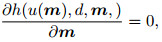
From Eq.(4), we can get

and

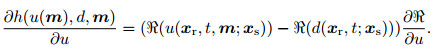
(7)

Applying the adjoint state method (Plessix, 2006), we can get the gradient,

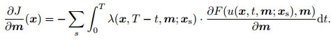
(8)

Here, the adjoint field λ=λ(x, tm; xs) is the solution of adjoint-equation,

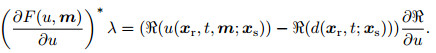
(9)

Here, symbol * is the adjoint operator and the right side of Eq.(9) is the adjoint source.

From Eq.(9), we can notice that the form of Eq.(9) remains the same for different physical problem, and we can use Eq.(9) to calculate the adjoint wavefield λ which acts as one time of seismic wave back propagation. Meanwhile, calculation of the term also needs another seismic wave simulation. It means that the inversion process based on misfit function of Eq.(4) is the same as conventional FWI, which needs two times of seismic wave simulation to calculate the gradient using Eq.(8) during each iteration.

Hence, we can conclude that the form of gradient and the adjoint state equation of waveform inversion based on different data subsets is the same as conventional FWI. The only difference is the adjoint source which depends on the physical problem, the form of misfit function and the data subsets. For example, the adjoint source for Eq.(4) is not only dependent on the residual of the synthetic and observed seismic data subsets, but also related to the operator .

The seismic data subset selected in the inversion is dependent on the characteristic of the field data and the stage of the inversion. Multi-step and multi-scale waveform inversion strategy can be realized by using different sub-kernel to calculate the gradient.

3 APPLICATIONS OF WAVEFORM INVERSION BASED ON SEISMIC DATA SUBSET

Theoretically, any physical information extracted from seismic data can be used as seismic data subset to implement above waveform inversion. There are three features that the data subset should satisfy. (1) It can reveal one or more characters of the seismic data; (2) It has specific physical meaning; (3) It can be extracted by some particular mathematical method.

Actually, some methods and strategies of FWI presented by some authors are more or less related to the idea of waveform inversion based on seismic data subset, and all their purpose is to reduce the nonlinearity of FWI by using part of seismic information. These data subsets can be selected as follows:

(1) The data subset is formed using some kinds of seismic phase. For example, if the operator is used to extract the waveform of the first arrivals, the corresponding inversion becomes first arrival waveform inversion (Sheng J et al., 2006) or the Gaussian beam first arrival waveform inversion (Liu et al., 2014). If the reflection waveform is extracted by operator , it becomes the reflection waveform inversion (Xu et al., 2012).

(2) The data subset is retrieved in a specific time window or a fixed observing aperture. For example, in order to reduce the nonlinearity of inversion, the operator can be treated as a window function. Then the above inversion method becomes the layer stripped waveform inversion (Wang et al., 2006; Yang et al., 2013). The operator also can be treated as an offset selection operator. Then the above inversion method becomes the offset selection waveform inversion strategy (Singh, 1989; Dong et al., 2013).

(3) The data subset is retrieved after some mathematical transforms. For example, if the operator stands for the Laplace transform, the data subset based waveform inversion will become the Laplace domain waveform inversion. Actually, the Laplace operator is applied to extract the first arrival time to robustly invert for a low wavenumber velocity model for the following inversion. If the operator is an integration operator, the above inversion method will degrade to the normalized integration waveform inversion method (Liu et al., 2011; Donno et al., 2013). With the normalized integrated seismic signal, FWI can provide us a good initial velocity model when low frequency is missing in the data and the initial model is poor. If the operator is selected as Hilbert transform to extract the envelope from the seismic data, the data subset based inversion will become the envelope based waveform inversion (Chi et al., 2013, 2014; Wu et al., 2014; Huang et al., 2015). A reliable initial model can be constructed by envelope based waveform inversion when the low frequency information is missing in seismic data. If we further combine the convolution and Hilbert transform as the operator , we can get the so-called source independent and envelope based waveform inversion (Ao et al., 2015). With such method, a good initial model can be inverted with unknown source wavelet, without low frequency in the data and no prior information about the subsurface model. And actually, the conventional multi-scale inversion strategy (Bunks et al., 1995; Sirgue and Pratt, 2004; Liu et al., 2012) also can be treated as a kind of data subset based waveform inversion, which firstly select low frequency data subset to invert for the background model and progressively increase the frequency content of the data subset to increase the resolution of the inversion result.

Besides, some special information in seismic data can form the data subset and can surely be applied in waveform inversion. For example, if the operator uses correlation to extract the first arrival time information, it is the wave equation first arrival time inversion (Luo and Schuster, 1991). If correlation is used to retrieve the reflected wave travel time, it is the reflection waveform inversion (Chi et al., 2015). And we gather all our courage to predict that if the operator is used to extract the reflected wave amplitude, the reflected wave amplitude inversion can be formed, which is similar to the AVO technology. Whether the gradient of this waveform inversion based on such certain information subset can be expressed as Eqs.(8) and (9) still needs further research.

The selection of seismic data subset is dependent on the stage of the inversion, the purpose of the inversion, and the character of the real seismic data. If the inversion target is the shallow part of the model, first arrival data subset can be selected for FWI. If the target is to provide a background velocity model for migration, the macro information in the seismic data can be selected as the data subset for FWI, such as travel time, envelope, data after Laplace transform, integrated data and phases. If the target is to get detailed description of the reservoir, the data subset should reveal the tiny variation of the data because only these faint data variations can reflect the change of the reservoir.

The inversion strategy we presented in this paper is a general idea, and it has different appearance in different situation. Dependent on what data subset used, some methods can invert for the long wavelength of the model and some for high resolution subsurface model.

If the target of FWI is to construct an accurate background model for migration, only part of the waveform information are needed to match rather than the full waveform information, and the nonlinearity of FWI surely can be reduced. If we aim to invert the low wavenumber components of the subsurface model by FWI, we should select the data subset which represents the macro variation of the data. Therefore, in the following part, three inversion tests based on data subsets are presented to illustrate how the seismic data subset based inversion goes and to prove the effectiveness of such strategy. Eq.(8) and (9) can be used to calculate the gradient of all data subset based waveform inversion methods. Here, we would not repeat it again.

One point we want to emphasize here is that the following three methods all based on the data subsets which stand for the macro character of the data, and the inversion results naturally present the large scale variation of the velocity model. In this sense, the three inversion methods we use here belong to the scope of velocity model building, and the results produced by these methods also prove this conclusion. However, comparing with the conventional model building methods (Al-Yahya, 1989; MacKay and Abma, 1992; Symes and Carazzone, 1991; Liu and Bleistein, 1995; Save and Fomel, 2003), the three presented in this paper are more automatic and do not need any manual interference.

3.1 An Example of Envelope Based Waveform Inversion

There are two challenges when applying FWI to field data. One is the lack of low frequency and the other is the poor initial model. Each of them can cause cycle-skipping problem during inversion. Meanwhile, the two are combined tightly together: more low frequencies are missing in seismic data, more accurate initial model is required for FWI. In other words, if a good subsurface model can be constructed by some other ways for FWI as initial model, the inversion results may still be acceptable even the low frequency information is missing in seismic data. Envelope of the seismic data retrieved by Hilbert transform is the macro character of the data and can be used to construct the objective function to invert for the low wavenumber of the velocity model. Envelope is one of the data subsets of seismic data and surely can use Eq.(8) and (9) to calculate the gradient for the envelope based waveform inversion.

Figures 1 and 2 are the results of Marmousi model test. Due to the lack of low frequencies below 5 Hz and the non-priori information initial model with constant gradient along depth (Fig. 1a), the result of conventional FWI is trapped in the local minima (Fig. 1b). However, under the same condition, the result of envelope based waveform inversion (Fig. 2a) is obviously much better, especially about the low wavenumber of the model. And taking such result as the initial model for the following conventional FWI, a high resolution result can be achieved finally without low frequency data and with the poor starting model.

Figure 3 is the initial model for a 2D survey line in South China Sea and its corresponding RTM migration result. Fig. 4 is the inversion result by the envelope based FWI and the corresponding RTM image. After envelope based FWI, the resolution of the model (Fig. 4a) is largely increased and the image is also improved a lot (Fig. 4b).

3.2 An Example of Elastic Envelope Inversion Without Low Frequency

Envelope reveals the macro characteristic of the seismic signal, and it can be used to invert for the low wavenumber of the velocity model. Recently, some good achievements are made by applying acoustic envelope FWI to single component seismic data to invert for the P-wave velocity model only (Chi et al., 2013, 2014; Wu et al., 2014).

For elastic full waveform inversion (EFWI) using multi-component seismic data, the two main challenges (low frequency missing and poor initial model) mentioned above still exist. Due to low S-wave velocity, much lower frequencies or more accurate initial model are required, which makes the EFWI even more difficult than acoustic FWI (Baeten, 2013; Brossier et al., 2009). To overcome these difficulties, we select the elastic envelope of multi-component data as the data subset to invert for the long wavelength components of the subsurface model. The final results show that this method can provide us good initial P-and S-model for the following conventional EFWI.

Figure 5 shows the true Marmousi-2 P-wave model and the initial P-wave velocity model used in EFWI. As the constant gradient starting models deviate substantially far from the true models and low frequencies below 5 Hz are filtered out, conventional EFWI suffers from cycle-skipping problem and fails to reach convergence (Fig. 6). In the results of the elastic envelope inversion (Fig. 7), however, the long-wavelength components of the subsurface models are well recovered. Then, after these results are used as the starting model for the subsequent conventional EFWI, the short wavelength components of the subsurface models are updated at the right positions and high resolution results are finally achieved (Fig. 8). This test proves that the two-step inversion method can achieve excellent results even when low frequency is missing in multicomponent data and initial model is far from the true model.

The vertical slices of the inversion results at the distance of X=7.5 km (Fig. 9) further indicate the advantage of the two-step inversion method. Above the depth of 2.2 km, the inversion result of two-step method is almost the same as the true model, but the result of conventional EFWI is far from the true model and is obviously trapped into local minima. Hence, when the low frequency is missing in multi-component data and the initial model is poor, applying elastic envelope based EFWI can well recover the long wavelength components of the subsurface model and provide a good initial model for the following conventional EFWI.

3.3 An Example of Reflection Waveform Inversion(RFWI)

In reflection seismology, the deep part of the model can only be reconstructed by reflections because only reflected waves can illuminate these areas. To overcome the cycle-skipping problem, a correlation-based criterion can be used to handle time delays between the synthetic and observed reflections, then the time delays can be used to define the misfit function. With such misfit function, the deep part of the background model can be well recovered. More specifically, the RFWI method is quite different from the conventional migration velocity analysis (MVA). The main advantage of the RFWI method is that it is a fully automatic velocity model inversion procedure in data domain.

The misfit function construction of the correlation-based reflection wave and the definition of the sub-kernel of reflected wave are crucial for the success of the RFWI. More details about this method can be referred to the reference (Chi et al., 2015). What we intend to show in this paper is the effectiveness of the waveform inversion based on seismic data subset by exhibiting the RFWI results in real data waveform inversion application.

A field data set acquired in East China Sea is used to test RFWI. Fig. 10a shows the smoothed velocity model constructed by pre-stack migration velocity analysis. The corresponding Gaussian-beam PSDM image is shown in Fig. 11. Fig. 10b exhibits the modifications of the velocity after RFWI with the smoothed model as initial model. The Gaussianbeam PSDM image with the inverted model is shown in Fig. 12. Comparing Fig. 11 with Fig. 12, the obvious improvement is achieved in the PSDM result obtained with the RFWI result. More detailed image of subsurface structures and more faults are revealed in Fig. 12. To further examine the accuracy of the inverted model, angle domain common-image gathers (ADCIGs) associated with the initial and final models are displayed in Fig. 13. The strong moveout in the ADCIGs (Fig. 13a) for the initial model indicates errors in the velocity model. However, after RFWI inversion, the flatter events in the ADCIGs (Figure 13b) indicate a more accurate model.

4 DISCUSSION

By analyzing the field data and selecting different data subset to construct misfit function with low nonlinearity at different inversion stages, we can realize the multi-step and multi-scale waveform inversion. Each step during this inversion procedure can be called the seismic data subset based waveform inversion. It is the objective requirement due to the complex relationship between the seismic data and the model parameters and the different inversion targets for different inversion stages during the seismic data processing and interpretation.

It is no doubt that someone may have such a question that ‘is it still the full waveform inversion?’ What is FWI? We all admit that the theoretical frame of FWI was presented by Tarantola (1984) and Lailly (1983), but they did not name their method as FWI. Instead, they preferred to treat it as data fitting. FWI first came out in the year of 1986 (Pan et al., 1986). In all the papers written by Tarantola, we cannot find the word of FWI, but nobody can deny his creative contribution on FWI. The main contribution of Tarantola to seismic data inversion is that he has set up the bridge between parameter inversion and migration under the idea of data fitting.

The final ideal for seismic inversion is to match all the information in seismic records. However, when dealing with real difficulty in different inversion stages, it is wise to lower the standard of inversion to fit with the reality and to match part of the information step by step rather than the whole information matching. This idea can be treated as seismic data subset based waveform inversion.

Hence, it is not necessary for us to define FWI as the full information matching process, because it may harm the flexibility and the development of FWI. However, if we define the FWI as the data subset matching method, it gives FWI more space to develop and more convenience to handle the practical problem.

5 CONCLUSION

(1) We present a generalized seismic data subset based waveform inversion method in this paper to deal with the strong nonlinearity of FWI and other difficulties occurred in practice. With different data subsets, the gradient of the misfit function has the same form and all can be calculated by forward and backward wave simulation. Only the adjoint sources are different for different physical problems, different data subsets and different forms of misfit functions.

(2) In the so-called seismic data subset based waveform inversion method, the idea of matching all seismic information should be abandoned. Conversely, different seismic data subsets should be used in this process on the basis of the analysis of the relations between different model parameters and different seismic data subsets at different FWI stages. And during the inversion, the back-projection of the selected data subset residual along the reasonable sub-kernel can decide which wavenumber and part of the model should be updated.

(3) Using the seismic envelope or the reflected wave information as seismic data subsets to construct a reasonable misfit function, we can well recover the long wavelength components of the subsurface velocity model, even if the low frequency is missing in the data and the initial model is poor. The synthetic and field data tests fully prove the effectiveness and accuracy of the data subset based inversion method.

ACKNOWLEDGMENTS

The authors greatly thank Prof. Jiubing Cheng and Dr. Tengfei Wang for providing PSDM algorithm used in the field data processing.