 2015, Vol. 58

 , SONG Sha-Lei1
 , LI Fa-Quan1, CHENG Xue-Wu1, CHEN Zhen-Wei1, LIU Lin-Mei1, YANG Yong1, GONG Shun-Sheng1
 2. University of Chinese Academy of Sciences, Beijing 100049, China
Temperature is an essential parameter of the atmosphere, which plays a key role in underst and ing the dynamical, radiative and coupling processes of different atmospheric layers. In the troposphere below 10 km, temperature is closely related to anthropogenic effects, which indirectly reflects the change of the ozone abundance(Wang et al., 2006). The tropospheric warming and stratospheric cooling reduce the vertical stability of the upper troposphere and lower stratosphere(UTLS)system because of the effects of greenhouse gases and ozone losses(Stohl et al., 2003). Moreover, wave-related variations, like the formation, propagation, and breaking of the tidal, planetary and gravity waves, strongly influence the temperature profile from the troposphere up to the upper mesosphere and thermosphere(Hauchecorne et al., 1992; Alpers et al., 2004; Rauthe et al., 2006). Thus, a connective detection of the Earth’s atmospheric temperature over a wide vertical range is of great significance for the study of the energy transmission in the atmosphere and the impact on the environment from anthropogenic behaviors.
To date, versatile lidar techniques have been developed especially for routine observations of the atmospheric temperature measurements with high precision and good temporal-spatial resolution. Based on different methodologies, temperature profiles are realizable from the ground up to the mesosphere and lower thermosphere(MLT). Absolute temperature above ~30 km can be accurately deduced from the relative air density due to Rayleigh scattering, assuming that the pure atmosphere is in a hydrostatic equilibrium and obeys the ideal gas law(Hauchecorne and Chanin, 1980; Whiteway and Carswell, 1995; Singh et al., 1996; Nee et al., 2002). When particles gradually contaminate Rayleigh signals, a vibrational Raman lidar that depends on a specificfrequency shift can be used instead to extend the temperature detection downward. While the weak cross section of the vibrational Raman and the interference of the aerosols, clouds and ozone concentration present considerable experimental difficulties for long range and high precision detection(Keckhut et al., 1990; Faduilhe et al., 2005; Wu et al., 2004). With a relatively stronger cross section than the vibrational Raman, the rotational Raman(RR)lidar is a method of choice for high-precision temperature measurements from the ground up to the stratosphere, even in the aerosol and optically cloud layers(Cooney, 1972; Arshinov et al., 1983; Liu et al., 2006; Achtert et al., 2013). However, it is still a challenge for the RR technique to measure the temperature accurately up to above 30 km, limited mainly by the weak signals 3~4 orders of magnitude smaller than the strong elastic backscattering. A large power-aperture product and sufficient suppression capacity(about 6~8 orders of magnitude)are important steps to obtain signal-to-noise ratios(SNR) and precision that are required. With the progress of the high-performance technologies in spectral extraction and weak signal detection, the temperature detection height for the RR lidar has been extended upward from an altitude of ~2 km(Cooney et al., 1976; Mao et al., 2009)to the stratosphere(Nedelijkovic et al., 1993; Behrendt and Reichardt, 2000; Behrendt et al., 2004; Achtert et al., 2013).
Temperature measurements covering from 1 to 105 km were performed at the Leibniz Institute of Atmospheric Physics with a combination of different lidars, in which the RR technique was used for altitudes below about 25 km. Their results encouraged the in-depth study of gravity graves(Alpers et al., 2004; Rauthe et al., 2006). The Esrange lidar combining RR measurements(5~35 km height) and the Rayleigh technique(30~80 km height)allowed for observations of small-scale temperature fluctuations to underst and the meteorological processes therein(Achtert et al., 2013). A newly reported RR lidar with a double-grating polychromater instead of narrowb and interference filters realized the temperature measurements at altitudes of 5~30 km. Jia and Yi(2014)have analyzed the relationship of the inversion layer and the temperature variability from the statistical results. They show that using the RR lidar to detect the temperature from the ground to the altitude above 30 km is of significance. Besides, to further link up with Rayleigh temperature, enough overlap is necessary to evaluate each method more timely and accurately.
This paper presents a PRR lidar system with a high-spectral resolution polychromator for high precision temperature measurements from 10~40 km over Wuhan. Temperature measurements up to 40 km by PRR lidar show the great potential for the further combination with the Rayleigh lidar. Observational results are compared with the local meteorological radiosondes, which show good consistency and reliability of the PRR lidar system. Temperature measurements from the ground up to 40 km cover the troposphere and most of the stratosphere, which lays a good foundation for the study of the dynamics and thermal dynamics in the medium-lower atmosphere.
2 PRINCIPLE OF RR TEMPERATURE MEASUREMENTThe principle for PRR temperature measurements is mainly based on the fact that the intensities of molecular rotational Raman lines exhibit different dependencies on temperature as a result of the Maxwell- Boltzmann distribution(Cooney, 1972; Penney et al., 1974). According to the selection rule of PRRS(△J = ±2), there exist two branches, the Stokes branch and the anti-Stokes branch, symmetrically located on the two sides of the incident light. Although the intensities of the Stokes branch are relatively stronger than those of the anti-Stokes branch, here we extract only the fractions of the anti-Stokes branch of the PRRS for temperature measurements to avoid the risk of interference of the Stokes branch with atmospheric fluorescence(Kitada et al., 1994). As shown in Fig. 1, the intensities of the low and high quantum transitions respectively decrease and increase as the temperature increases.

|
Fig.1 Anti-Stokes branch of pure rotational Raman spectrum of molecular nitrogen and oxygen at T=280 K and T=200 K. The laser wavelength is set at 532.1 nm in air. RR1 and RR2 are two regions of opposite temperature dependence. |
To determine the relationship and finally invert the temperature, two domains(RR1 and RR2 channels) with opposite temperature sensitivities are extracted from the anti-Stokes branch of the RR spectrum. The RR signals denoted by the lidar equation is

where S0 is the number of transmitted photons; A is the free telescope area; O(z) is the overlap between
transmitted laser and telescope; △z is the height resolution; N(z) is the spatial density of air molecules; τ atm2is the atmospheric roundtrip transmission; "ε is the detector efficiency; ηi is the relative volume abundance of N2 and O2, respectively; τRR(Ji)is the filter transmission at the wavelength of the RRS line Ji; and  is the differential backscatter cross section for the single line of the RR spectrum.
By taking the ratio of the two RR channel signals, all light intensity related parameters(e.g. the laser power, telescope area, air density and the atmospheric extinction)can be neglected(Fraczek et al., 2013). It is only the RR spectral intensity and the specific filter parameters that affect the signal’s ratio for temperature determination.
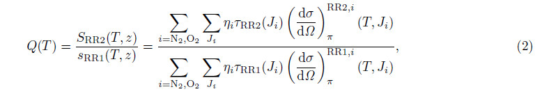
where Q is the signal ratio; and SRR1 and SRR2 are the detected signals from the RR channel of the low and high quantum transitions, respectively. Temperature can be inverted with the calibration function(Behrendt, 2005)as follow

where a, b, c are the calibration coefficients. RR temperature is generally calibrated by comparison with data measured with other instruments such as local radiosondes. Of course, the reference data used for the calibration should be taken as close in space and time as possible to the atmospheric column sensed by the lidar. With an initial calibration for the lidar-derived temperature profile, no further calibration is necessary in the case of a stable performance of the lidar system.
3 SIMULATION OF FILTER PARAMETERS IN RR CHANNELSOn one h and , the spectral distribution and specific filter parameters determine the temperature dependence of RR lidar detection. Thus, a high-spectral resolution polychromator for light splitting and filtering is necessary. On the other h and , as the Raman-shifted return signals are 3~4 orders of magnitude less than the Rayleigh-Mie return, sufficient suppression of the elastic backscatter signals(6~7 orders of magnitude)in the RR detection channels must be satisfied. Thus the state of the art interference filters are selected to realize the signal separation with high spectral resolution.
With the development of filter technology, multi-cavity interference filters possess the advantages of ultranarrow b and width, high transmittance, high b and rejection capabilities and excellent temperature insensitivity. Besides, their center wavelength and b and width can be tuned while changing the angle of the interference filters. In this section, the central wavelength(CWL) and full-width-at-half-maximum b and width(FWHM)of the filters are two main parameters considered in simulated calculation. The optimal selection of the filter CWL and FWHM provides a theoretical reference for the subsequence system design and operation.

In the simulation, the laser wavelength is at 532.1 nm. The atmospheric temperature is assumed ranging from 200 K to 280 K. By changing the CWL from 528 nm to 532 nm and FWHM from 0 to 3 nm, the temperature sensitivity of the signal intensity, defined by Eq.(4), is shown in Fig. 2a. The two opposite temperature dependence regions are evidently distinguished at the wavelength of ~530.2 nm. Positive values as noted in the color bar represent the positive correlation of the signal and the temperature, while the negative shows the negative correlation. For simplicity, the transmission curve of the filter is assumed rectangular-shaped and the peak transmission τ = 1 while for the out-of-b and transmission τ0. Calculation step width is 0.01 nm. The most sensitive places as shown in Fig. 2a are around CWL1=531.03 nm, FWHM1 = 1.44 nm, CWL2 = 528.8 nm, FWHM2=3.0 nm, respectively.

|
Fig.2 (a) Temperature dependency of the calculated signals for filters with different central wavelengths (CWL) and channel passbands (FWHM); (b) Simulated calculations of the temperature measurement uncertainty for different center wavelengths in the two rotational Raman channels with filter bandwidths of 0.7 nm and 1.1 nm |
As the lidar photon-counting signals follow Poisson statistics, the 1-σ statistical error is proportional to the inverse square root of the number of photons detected. The uncertainty of the RR temperature measurements (Behrendt et al., 2005)is given by

The statistical temperature uncertainty of the RR technique is related to both the temperature sensitivity and the signal intensity. Thus, when selecting the proper filter b and widths and center wavelengths, both the temperature sensitivity and the signal intensity should be taken into account to minimize the measurement uncertainty. Since the CWL of RR1 channel is closer to the laser wavelength, a narrower b and width filter is considered to suppress the elastically scattered signal; while for the RR2 channel the b and width can be relatively wider for extracting strong enough signals. When setting the b and widths of the two RR channels at 0.7 nm and 1.1 nm, calculation results about the temperature uncertainty versus the CWL of both RR channels are shown in Fig. 2b. The white box indicates that the smallest temperature uncertainty is around the theoretically optimal CWLs of 531.39~531.45 nm and 528.5~528.7 nm, where the lowest temperature uncertainty is set as △Toptimum = 1.
In practical application, however, it is almost impossible to achieve the same parameters(peak transmission and out-of-b and blocking)as those in the theoretical simulation. Besides, the filter parameters must be adjusted as the laser wavelength or line width changes a little. Thus, the optimal design of the light separating and receiving system of the RR lidar need depend on the simulation analysis.
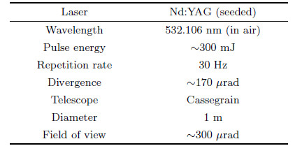
4 ROTATIONAL RAMAN LIDAR SYSTEMFigure 3 shows the schematic overview of the RR lidar system whose main characteristics are presented in Table 1. A frequency-doubled and seeded-injection Nd: YAG laser is used as a transmitter to emit light at 532.1 nm in the air with 300 mJ pulse energy at a repetition frequency of 30 Hz. Exp and ed by a beam widening telescope, the laser beam with a divergence of ~170 μrad is directed vertically into the atmosphere. Signals backscattered from the atmosphere are collected by a Cassegrainian telescope with a diameter of 1 m and transferred into the beam collimating and splitting system through an optical fiber. Finally two RR signals are captured by a transient reorder(Licel) and stored in a computer for later data processing.

|
Fig.3 Schematic setup of the rotational Raman lidar Table 1 Technical parameters of the rotational Raman lidar |
| Table 1 Technical parameters of the rotational Raman lidar |
The laser wavelength selected in the lidar system is mainly considering for the temperature and wind joint observation on the basis of two mechanisms of Raman and Rayleigh scattering. After laser beam expansion and collimation, rigorous match of the light receiving and transmitting, high-resolution light splitting and filtering and the weak-signal detection technique, not only the overall system performance can be improved, temperature data at high altitudes with more precision can also be guaranteed.
The key technology of the RR lidar system design is to achieve the high-resolution light splitting and filtering for the two RR channels. Design of the light splitting and filtering system for the RR lidar is shown in Fig. 4a. Signals collected from the telescope are first collimated by a set of combined lenses. Considering thatthe filter performance changes with the angle of incidence, a higher level of collimation is required for the Z-shaped separating light path as long as 1.5 m. Fig. 4b shows the collimated system that consists of three lenses and an effective focal length of 73 mm. The Z-shaped optical design spectrally realizes the light separating of Raman and elastic scattering signals with the help of high-performance interference filters. The transmittance profiles of the tested filters are plotted in Fig. 4b. The filters in the two RR channels are centered at the wavelengths of 530.9 nm and 528.9 nm with the b and widths of 0.7 nm and 1.1 nm, respectively. Compared with the above simulation results, the temperature measurement uncertainty under these tested filter parameters is △T = 1.1×△Toptimum, which is close to the optimal position.

|
Fig.4 Design of the light splitting and filtering system for rotational Raman lidar (a) Optical path of the light splitting and filtering; (b) Collimating system; (c) Transmittance profiles of the tested filters. Fig. 5 Raw received signals of the rotational Raman lidar |
Since established in March 2014, the PRR temperature measurement lidar has been operated for nocturnal observations over Wuhan, China(30.5°N, 114.4°E). By data inversion, a total of ~300 hours of temperature profiles were collected from the altitude of 10 km to 40 km. In order to validate the reliability of lidar performance, the measured temperature profiles were compared with local radiosondes. The good agreement and high precision verified the feasibility of the lidar system.
5.1 Temperature Measurement of Lidar and Comparison with RadiosondesFigure 5 shows the 1 h-integrated signal profiles(background-corrected)received separately from the RR1 and RR2 channels with a range resolution of 300 m. The local time(LT)is 20:00-20:56, on 4 June 2014. With the bi-axial configuration of the laser emitter and telescope receiver, the stronger signals at lower altitudes below ~10 km are effectively restrained, which ensures the detection quality of the weaker signals at higher altitude up to 40 km.

|
Fig.5 Raw received signals of the rotational Raman lidar |
Based on the received signals shown in Fig. 5, the temperature profile from 10~40 km measured by PRR lidar is plotted in Fig. 6a together with the temperature profile from the local radiosonde. The launch time for the local radiosonde is 20:00 LT, which is close to lidar measurements in space and time. Thus the calibration can be done for the temperature retrieval.Fig. 6b shows the statistical temperature errors of the lidar measurement and the temperature deviations between lidar and radiosonde. It can be seen that temperature measured by the PRR lidar agrees well with the local radiosonde temperature. By subtracting the lidar temperature ofradiosonde’s, the maximum temperature deviation is no more than 3.0 K for altitudes below 30 km. The good consistency confirms the reliability of the PRR lidar. While above 30 km, the large temperature deviation may be caused by both the increasing statistical error of the lidar measurements and the limited capability for the radiosondes(Chen, 2010; Zhang et al., 2013). With the 1 h integration and 300 m spatial resolution, the statistical temperature error for PRR lidar increases from 0.4 K at 10 km up to about 8 K at the altitude close to 40 km. There exists a difference of about 20 times for the statistical errors detected at the high and low altitudes. The tempora or spatial resolution must be lowered for smaller temperature errors especially at high altitudes. Thus, a trade-off between the measurement precision and the temporal and spatial resolution must be satisfied.

|
Fig.6 (a) Temperature profiles measured by the rotational Raman lidar (solid line) in comparison with the simultaneous radiosonde (circles). Error bars show the statistical errors of the lidar measurement; (b) Statistical errors of the lidar measurement (solid line) and the temperature deviations between lidar and radiosonde (circles) |
The status and characteristics of the atmosphere change significantly with height. The higher light goes above the earth, the thinner the air is. Lidar signal intensity is not only inversely proportional to the square of the height but also closely related to atmospheric attenuation. Thus, signal-to-noise ratios(SNR)are very different for signals received from different altitudes, which directly determines the temperature measurement uncertainties. In the data processing, varying spatial resolutions for different altitudes are generally used to narrow the gap of statistical errors.
Figure 7a shows a combined temperature profile obtained on 4 April 2014 with 60 min time integration and varying spatial resolutions for different altitudes. The spatial resolution is 150 m for altitudes from 10~20 km, 450 m for 20~30 km and 750 m for 30~40 km. As shown in Fig. 7b the corresponding statistical errors for different ranges are about 0.3 K, 0.7 K and 2.3 K(They are the average of the statistical temperature errors in different detection ranges).

|
Fig.7 (a) Combined temperature profile with 60 min integration and different spatial resolutions for different altitudes (the solid line is for 10~20 km with 150 m resolution, the dashed line is for 20~30 km with 450 m resolution, and the dotted line is for 30~40 km with 750 m resolution). Error bars show the statistical errors of the lidar temperature; (b) Statistical temperature errors of the lidar measurement for different altitudes with different spatial resolutions (solid line) and the temperature deviations between lidar and radiosonde (circles) |
Considering that some fluctuations in the atmosphere change quickly with very short periods, the detection of rapid changes from stable temperature profiles is necessary in order to capture some subtle messages. Therefore, temperature measurement with high temporal resolution will help to research the wave phenomena and microphysical properties. To simultaneously ensure the SNR and precision of the temperature measurement, spatial resolutions are still required to be varying in different heights. Take the same night of Fig. 7 for example. The integration time is reduced to 30 min as shown in Figs. 8a and 8b. The spatial resolutions are adjusted to 300 m, 600 m and 900 m for altitudes of 10~20 km, 20~30 km and 30~40 km, and correspondingly, thestatistical errors for different ranges become ~0.3 K, 0.8 K and 3.0 K. In Figs. 9a and 9b, the integration time is 10 min and the spatial resolutions are separately 450 m, 750 m and 1200 m for altitudes of 10~20 km, 20~30 km and 30~40 km. Statistical errors for different ranges are ~0.4 K, 1.1 K and 3.8 K. The high precision under a high temporal resolution will contribute to the study of the minor fluctuations with small amplitudes or short cycles.

|
Fig.8 (a) Combined temperature profile with 30 min integration and different spatial resolutions for different altitudes (the solid line is for 10~20 km with 300 m resolution, the dashed line is for 20~30 km with 600 m resolution, and the dotted line is for 30~40 km with 900 m resolution). Error bars show the statistical errors of the lidar temperature; (b) Statistical temperature errors of the lidar measurement for different altitudes with different spatial resolutions (solid line) and the temperature deviations between lidar and radiosonde (circles) |

|
Fig.9 (a) Combined temperature profile with 10 min integration and different spatial resolutions for different altitudes (the solid line is for 10~20 km with 450 m resolution, the dashed line is for 20~30 km with 750 m resolution, and the dotted line is for 30~40 km with 1200 m resolution). Error bars show the statistical errors of the lidar temperature; (b) Statistical temperature errors of the lidar measurement for different altitudes with different spatial resolutions (solid line) and the temperature deviations between lidar and radiosonde (circles) |
What is common in Figs. 7-Fig. 9b is that temperature deviations between the lidar and radiosonde are found very small(< 3 K)below 25 km, but increases obviously above 25 km(the maximum being ~8 K). On one h and , because the radiosonde has drifted far away from the lidar site and its detection ability at high altitudes around 30 km cannot be guaranteed. On the other h and , temperature deviations between the lidar and radiosonde will increase unexpectedly especially when some special atmospheric phenomena appear, like the temperature inversion
5.3 Continuous Temperature Profiles all the NightFigure 10a shows the whole night temperature profiles observed from 21:42 on 4 August 2014 to 05:08 on 5 August 2014. The temporal resolution is 30 min, and the spatial resolution is 300 m for altitudes from 10~20 km, 600 m for 20~30 km and 900 m for 30~40 km. As the lidar system worked stably, the temperature was obtained with the initial calibration on 22 July 2014. When comparing the lidar-derived temperature with the radiosonde temperature data released at 20:00 LT on 4 August, the deviation is no more than 3 K from 10~30 km. Besides, the lidar temperature on the morning of 5 August also agrees well with the radiosonde temperature released at 08:00 LT on 5 August. Although lidar temperature is a little lower than the radiosonde’s, their deviations from 10~20 km are less than 2 K and the maximum at 30 km is about 5.3 K. The excellent agreement between the lidar and radiosonde demonstrates that the PRR lidar system can continuously and steadily work with long-term dependability.

|
Fig.10 (a) Temperature profiles (solid lines) measured by rotational Raman lidar from 21:42 on August 4, 2014 to 05:08 on August 5, 2014. The circles are the temperature data released by the local radiosonde at 20:00 LT on August 4 and at 08:00 LT on August 5; (b) Time-height contour of the temperature profiles observed all night long |
The thermal structure in the medium-lower atmosphere from 10~40 km can be seen from the time-height contours of the temperature profiles during the whole night(Fig. 10b). At the very beginning, temperature in the troposphere decreases with height. At the tropopause of around 18 km, a minimum temperature of ~195 K occurs. Then temperature increases when entering into the stratosphere. With the high space-time resolution and high accuracy temperature detection, more detailed analysis of the fluctuations will be helpful to study the dynamic processes of the atmosphere.
6 CONCLUSIONSThis paper describes the system design and observational results of a PRR lidar for the temperature measurements from 10~40 km over Wuhan. Based on an injection-seeded laser source and an 1 m diameter telescope, state of the art interference filters for light splitting and filtering were designed to extract the required PRR signals and suppress the elastically backscattered light. With the optimum design of optical spectroscopy parameters, as well as exact light receiving and transmitting match, PRR scattering returns were detected by the weak signal detection technology. Lidar observational results are presented to investigate the overall lidar performance. Compared the temperature profiles simultaneously measured by the PRR lidar and the local meteorological radiosonde, the maximum deviation below 30 km is about 3.0 K, which shows good consistency and reliability of the PRR lidar system. Obvious deviations may occur because of the balloon drifts, regional difference and special phenomenon like the thermal inversion layer. Temperature profiles at different temporal scales(10 min, 30 min and 60 min)are given for analysis of the wave properties and microstructures. The statistical temperature errors vary with the spatial resolutions in different detection ranges. For the 30 minintegrated lidar temperature profile, the statistical error is about 0.3 K for altitudes of 10~20 km with 300 m spatial resolution; about 0.8 K for altitudes of 20~30 km with 600 m resolution; while with the 900 m spatial resolution, it is about 3.0 K for altitudes from 30 km up to 40 km. In addition, the whole night temperature profiles are given in this paper, which demonstrate the long-term dependability of the PRR lidar system and provide an effective detection means for detailed analysis of the atmospheric dynamic processes. Temperature measurement up to 40 km by PRR lidar possesses great potential for the further combination with the Rayleigh lidar of 30~80 km detection capacity. Besides, the combination with the narrow laserb and resonance fluorescence lidar technique covering from 80~110 km will finally realize the whole atmospheric temperature detection from the ground up to 110 km.
ACKNOWLEDGMENTSWe acknowledge the Wuhan Weather Station for providing the radiosonde data. This work was supported by the National Natural Science Foundation of China(41127901, 41101334, 11403085).
| [1] | Achtert P, Khaplanov M, Khosrawi F, et al. 2013. Pure rotational-Raman channels of the Esrange lidar for temperature and particle extinction measurements in the troposphere and lower stratosphere. Atmospheric Measurement Techniques, 6(1): 91-98, doi: 10.5194/amt-6-91-2013. |
| [2] | Alpers M, Eixmann R, Fricke-Begemann C, et al. 2004. Temperature lidar measurements from 1 to 105 km altitude using resonance, Rayleigh, and Rotational Raman scattering. Atmos. Chem. Phys., 4(3): 793-800, doi: 10.5194/acp-4-793-2004. |
| [3] | Arshinov Y F, Bobrovnikov S M, Zuev V E, et al. 1983. Atmospheric temperature measurements using a pure rotational Raman lidar. Appl. Opt., 22(19): 2984-2990, doi: 10.1364/AO.22.002984. |
| [4] | Behrendt A, Reichardt J. 2000. Atmospheric temperature profiling in the presence of clouds with a pure rotational Raman lidar by use of an interference-filter-based polychromator. Appl. Opt., 39(9): 1372-1378, doi: 10.1364/AO.39.001372. |
| [5] | Behrendt A, Nakamura T, Tsuda T. 2004. Combined temperature lidar for measurements in the troposphere, stratosphere, and mesosphere. Appl. Opt., 43(14): 2930-2939, doi: 10.1364/AO.43.002930. |
| [6] | Behrendt A. 2005. Temperature Measurements with Lidar. //Weitkamp C E ed. Lidar: Range-Resolved Optical Remote Sensing of the Atmosphere. New York: Springer, 102: 273-305. |
| [7] | Chen Z. 2010. Characteristics of the overall sounding data drift in China. Meterological Monthly (in Chinese), 36(2): 22-27. |
| [8] | Cooney J. 1972. Measurement of atmospheric temperature profiles by Raman backscatter. J. Appl. Meteor., 11(1): 108-112, doi: 10.1175/1520-0450(1972)011¡0108:MOATPB¿2.0.CO;2. |
| [9] | Cooney J, Pina M. 1976. Laser radar measurements of atmospheric temperature profiles by use of Raman rotational backscatter. Appl. Opt., 15(3): 602-603, doi: 10.1364/AO.15.000602. |
| [10] | Faduilhe D, Keckhut P, Bencherif H, et al. 2005. Stratospheric temperature monitoring using a vibrational Raman lidar, Part 1: Aerosols and ozone interferences. J. Environ. Monitor., 7(4): 357-364, doi: 10.1039/B415299A. |
| [11] | Fraczek M, Behrendt A, Schmitt N. 2013. Short-range optical air data measurements for aircraft control using rotational Raman backscatter. Optics Express, 21(14): 16398-16414, doi: 10.1364/OE.21.016398. |
| [12] | Hauchecorne A, Chanin M L. 1980. Density and temperature profiles obtained by lidar between 35 and 70 km. Geophys. Res. Lett., 7(8): 565-568, doi: 10.1029/GL007i008p00565. |
| [13] | Hauchecorne A, Chanin M L, Keckhut P, et al. 1992. LIDAR monitoring of the temperature in the middle and lower atmosphere. Appl. Phys. B, 55(1): 29-34, doi: 10.1007/BF00348609. |
| [14] | Jia J Y, Yi F. 2014. Atmospheric temperature measurements at altitudes of 5-30 km with a double-grating-based pure rotational Raman lidar. Appl. Opt., 53(24): 5330-5343, doi: 10.1364/AO.53.005330. |
| [15] | Keckhut P, Chanin M L, Hauchecorne A. 1990. Stratosphere temperature measurement using Raman Lidar. Appl. Opt., 29(34): 5182-5186, doi: 10.1364/AO.29.005182. |
| [16] | Kitada T, Hori A, Taira T, et al. 1994. Strange behaviour of the measurement of atmospheric temperature profiles of the rotational Raman lidar. //17th International Laser Radar Conference, National Institute for Environmental Studies, Tsukuba, Japan. |
| [17] | Liu Y L, Zhang Y C, Su J, et al. 2006. Rotational Raman lidar for atmospheric temperature profiles measurements in the lower-air. Opto-Electronic Engineering (in Chinese), 33(10): 43-48. |
| [18] | Mao J D, Hua D X, Wang Y F, et al. 2009. Accurate temperature profiling of the atmospheric boundary layer using an ultraviolet rotational Raman lidar. Opt. Commun., 282(15): 3113-3118, doi: 10.1016/j.optcom.2009.04.050. |
| [19] | Nedelijkovic D, Hauchecome A, Chanin M L. 1993. Rotational Raman lidar to measure the atmospheric temperature from the ground to 30 km. IEEE Trans. Geosci. Remote Sens., 31(1): 90-101, doi: 10.1109/36.210448. |
| [20] | Nee J B, Thulasiraman S, Chen W N, et al. 2002. Middle atmospheric temperature structure over two tropical locations, Chung Li (25°N, 121°E) and Gadanki (13.5°N, 79.2°E). J. Atmos. Solar-Terr. Phys., 64: 1311-1319, doi:10.1016/S1364-6826(02)00114-1. |
| [21] | Penney C M, St Peters R L, Lapp M. 1974. Absolute rotational Raman cross sections for N2, O2 and CO2. Journal of the Optical Society of America, 64(5): 712-716, doi: 10.1364/JOSA.64.000712. |
| [22] | Rauthe M, Gerding M, Hffner J, et al. 2006. Lidar temperature measurements of gravity waves over Kühlungsborn (54°N) from 1 to 105 km: A winter-summer comparison. J. Geophys. Res., 111: D24108, doi: 10.1029/2006JD007354. |
| [23] | Singh U N, Keckhut P, McGee T J, et al. 1996. Stratospheric temperature measurements by two collocated NDSC lidars during UARS validation campaign. J. Geophys. Res., 101(D6): 10287-10297, doi: 10.1029/96JD00516. |
| [24] | Stohl A, Bonasoni P, Cristofanelli P, et al. 2003. Stratosphere troposphere exchange: A review, and what we have learned form STACCATO. J. Geophys. Res., 108(D12): 8516, doi: 10.1029/2002JD002490. |
| [25] | Wang W G, Fan W X, Wu J, et al. 2006. A study of spatial-temporal evolvement of the global cross-tropopause ozone mass flux. Chinese J. Geophys. (in Chinese), 49(6): 1595-1607, doi: 10.3321/j.issn:0001-5733.2006.06.004. |
| [26] | Whiteway J A, Carswell A I. 1995. Lidar observations of gravity wave activity in the upper stratosphere over Toronto. J. Geophys. Res., 100(D7): 14113-14124, doi: 10.1029/95JD00511. |
| [27] | Wu Y H, Hu H L, Hu S X, et al. 2004. Rayleigh-Raman scattering lidar for atmospheric temperature profiles measurements. Chinese Journal of Lasers (in Chinese), 31(7): 851-856. |
| [28] | Zhang L, Liu Q Q, Yang R K, et al. 2013. A method based on the computational fluid dynamics for solar radiation error correction of sounding temperature sensors. Chinese Journal of Sensor and Actuators (in Chinese), 26(1): 78-83. |