1 INTRODUCTION

With the development of exploration technologies, seismic anisotropy has been observed in many exploration areas, especially in sedimentary rocks. Transverse isotropy(TI)with a vertical symmetry axis(VTI)canprovide a good representation of intrinsic anisotropy induced by horizontally aligned parallel fractures and finelaminations. Reverse time migration for anisotropic media based on the full anisotropic elastic wave equationis computationally inefficient and requires at least five parameters. On the other h and , conventional P-waveseismic data, gathered at the earth’s surface, contain only the vertical component of the elastic wave. So, forpractical application of anisotropy, transverse isotropy is commonly adopted under the acoustic approximation.

In general, we can divide these acoustic approximations into two broad categories:(a)the coupled pseudoacoustic wave equations(Alkhalifah, 2000; Zhou et al., 2006; Hestholm, 2009; Fletcher et al., 2009; Fowler et al., 2010; Duveneck and Bakker, 2011; Zhang et al., 2011) and (b)the decoupled pure P-wave equations(Klié and Toro, 2001; Etgen and Br and sberg-Dahl, 2009; Liu et al., 2009; Crawley et al., 2010; Pestana et al., 2011; Chu et al., 2011, 2013; Zhan et al., 2011, 2013; Huang et al., 2011). The pseudo-acoustic equations areusually derived from the exact P-SV dispersion relation, simplified by setting the shear-wave velocity to zero(Alkhalifah, 2000). Although pseudo-acoustic wave equations yield kinematically accurate P-wave propagation, all these wave equations contain undesired shear-wave artifacts(Grechka et al., 2004). In addition, the pseudoacoustic wave equations become numerically unstable for anisotropic models with anisotropic parameters ε < δ.For these above mentioned reasons, the decoupled pure P-wave equations for modeling and migration in TImedia have attracted more attentions. The pure P-wave equations are also derived from the exact dispersionrelation by using a Taylor, Pad′e, or similar expansion to replace the square root with or without setting theshear-wave velocity to zero. The pure P-wave equations usually involve fractional pseudo-differential operatorsthat make the numerical implementation difficult when using the finite-difference(FD)method alone. The mostnatural choice to solve these equations is pseudospectral(PS)method(Kosloff and Baysal, 1982; Reshef et al., 1988a, 1988b). Besides, some other modified spectral methods are used to solve those special pure P-wave equations(Etgen and Br and sberg-Dahl, 2009; Crawley et al., 2010, Crawley Pestana and Stoffa, 2010). Although PSmethod requires only two nodes per wavelength, it is still computationally expensive because several fast Fouriertransforms(FFTs)are required in wavefield extrapolation at each time step. Zhan et al.(2013)proposed anefficient hybrid PS/FD scheme for solving second-order TTI pure P-wave equation.

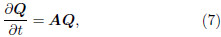
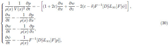
Here, we propose the first-order form of the pure P-wave equation with stress and particle velocities aswavefield variables for heterogeneous VTI media. And we adopt the similar method to solve the proposed firstorder equation using hybrid PS/FD scheme. The proposed methods extend the pure P-wave equations fromthe cases of constant density to those of variable density. Moreover, another advantage of the velocity-stressequation is that we can use high-order staggered-grid finite difference in our numerical implementation to reducethe grid dispersion.

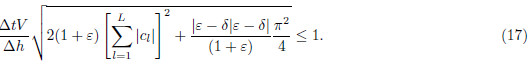
Stability of seismic numerical wave modeling is a dem and ing topic. The stability analysis for numericalsolutions of partial derivative equations is usually h and led using the von Neumann’s method. In numericalimplementation, spatial sampling is generally chosen to avoid grid dispersion in solutions and the temporalsampling is chosen to avoid numerical instability(Lines et al., 1999). The stability of the hybrid PS/FD schemeon central and staggered grids is investigated in this paper. The analysis shows that the staggered-grid hybridPS/FD scheme is more stable than central-grid hybrid PS/FD scheme. The hybrid PS/FD scheme on centralgrid is unstable when the anisotropy parameter is greater than δ. This instability problem is restricted towavenumbers near Nyquist. To deal with this problem, a low-pass filter is applied to the wavenumber operatorsin our numerical implementation.

2 VTI PURE P-WAVE EQUATION

We start our derivation from the exact VTI phase velocity expression(Tsvankin, 1996):

where θ is phase angle, ε and δ are Thomsen parameters(Thomsen, 1986), f =, V_P0 and V_S0 representthe P- and SV-wave velocities along the symmetry axis, respectively. Here, the plus sign corresponds to the Pwave and the minus sign to the SV wave. Letting VS0 = 0, then Eq.(1)reduces to

We only consider the plus sign. Using first-order Taylor expansion to replace the square root of Eq.(2)gives the following approximation for the P-wave phase velocity(Klié and Toro, 2001; Fowler, 2003):

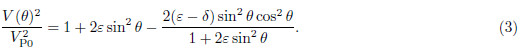
Figure 1 displays a comparison between the exact phase velocity(black dotted line) and the approximatephase velocity(gray solid line)governed by Eq.(3)with V_P0 = 3500 m·s^-1, V_S0 = 2023 m·s^-1 and anisotropyparameter(a)ε = 0.2, δ = -0.1, (b)ε = 0.05, δ = 0.3. Fig. 1c is the maximum relative errors of approximateP-wave phase velocity compared to the exact P-wave phase velocity for different anisotropy parameters ε varyingfrom 0 to 0.4 and ε varying from –0.2 to 0.4. Fig. 2 displays the maximum relative errors of approximate P-wavephase velocity for the effective anisotropy parameter η(Alkhalifah and Tsvankin, 1995). Fig. 1 and Fig. 2 showsthat the approximate P-wave phase velocity is very close to the exact phase velocity. For weak anisotropy(i.e. < 0.2), the relative phase velocity errors are below 1%. Note that Fig. 1c and Fig. 2 also indicate thatstrong anisotropy may lead to large error. Generally speaking, pure P-wave equation gives a reasonably good approximation to the exact phase velocity for weak anisotropy, but the accuracy decreases with the increase ofanisotropy.

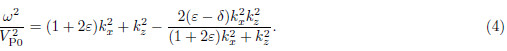
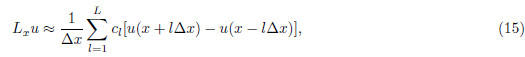
Plugging the relations sin θ = and cos θ = , where ω is angular frequency, k_x and k_zare spatial wavenumbers in x and z directions, into Eq.(2)gives the following VTI pure P-wave approximatedispersion relation(Fowler, 2003; Chu et al. 2011):

A clearer relation between two approximate dispersion relations of pseudo-acoustic wave and pure P wave isdiscussed in Appendix. Applying an inverse Fourier transform to both sides and then using the Fourier transformproperties -iω → ∂/∂t, ik_x→ ∂/∂x and ik_z → ∂/∂z, we finally obtain the following time-space-domain pureP-wave equation:

where F [ ] and F ^-1[ ] represent forward and backward Fourier transform, respectively, , i is square root of –1. Letting auxiliary wavefield , we can obtain a hyperbolic system of first-orderequations as

where ρ is density. By analogy with the velocity-stress formulation of the isotropic acoustic wave equation, u and w represent particle velocities. The auxiliary wavefield ψ in the system of Eq.(6)vanishes in the case ofelliptical anisotropy(ε = δ). If ε = δ = 0, Eq.(6)reduces to the acoustic isotropic wave equation, the solutionof which is the pressure wavefield.

3 STABILITY

The stability problem is a very important aspectin seismic wave numerical simulations. Because of thefractional pseudo-differential operators, the stability offirst-order pure P-wave equation may be different fromthe isotropic acoustic or elastic equations. In this section, we focus our work on the stability analysis of thehybrid PS/FD scheme on central and staggered grids.

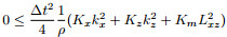
Eq.(6)takes the form as the following hyperbolicwave equation:

where , and

Taking the derivative of Eq.(7)with respect to t, we obtain

where

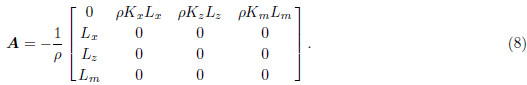
Replacing the time derivative of Eq.(9)with a second-order FD scheme, and applying spatial and temporalforward Fourier transform to wavefiled Q, we obtain

where , I is identity matrix, and

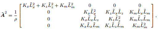
where .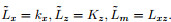

Since is a hyperbolic equation, there exists a nonsingular matrix S such that , where Λis a positive diagonal matrix composed of eigenvalues λi(Dong et al., 2000)of matrix , and then

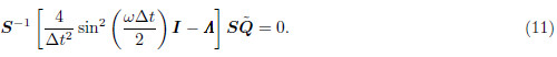
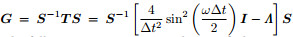Letting , then det(G)= det(T). If Eq.(11)has non-zerosolution, the following expression must be satisfied

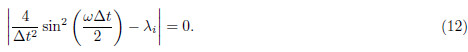
Since , we obtain the stability condition as

Numerical implementation is stable if and only if the two inequalities in expression(13)are satisfied.

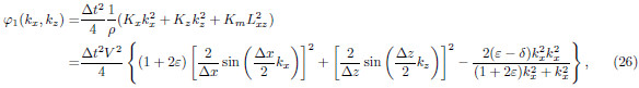
We first discuss the inequality . The eigenvalues of matrix are λ₁ = λ₂ = , and λ₃ = λ₄ = 0. Since the sign of Km is uncertain, we use the following inequality

Consider a function u(x)which has a continuous first derivative. The 2L-order central-difference approximationto first derivative is

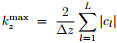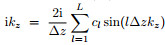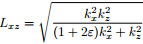
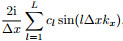
where cl(l = 1, 2, · · ·, L)are FD coefficients. Substituting an harmonic plane wave into Eq.(15), we obtain ik_x =, and . Similarly, we have and 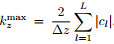. We use PS method to calculate the fractional pseudo-differential operators. Thesampling theorem tells us that and . Therefore the maximum value of L_xz is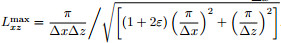. Plugging k_x ^max, k_z ^max and L_xz^max into inequality(14)yields

For the special case Δx = Δz = Δh, the stability condition reduces to

Then we investigate the staggered-grid hybrid PS/FD scheme. The 2L-order staggered-grid finite-differenceapproximation to first derivative is

where a_l(l = 1, 2, 3, · · ·, L)are SGFD coefficients. Fig. 3 shows the elementary cell of 2D staggered-grid schemein which pressure wavefield, particle velocities, density and anisotropic parameters are defined. Since the derivation is similar to central-grid case, we directly give the stability condition of staggered-grid hybrid

For the special case Δx = Δz = Δh, the stability conditionreduces to

If anisotropic parameters are zeros, stability conditions(17) and (20)reduce to the isotropic acoustic case.

Next, we discuss the other inequality . As discussed above, the following inequality has to besatisfied

If K_m ≥ 0, then . So we only investigate the case where K_m < 0. Let

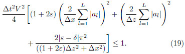
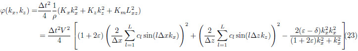
For central-grid finite-difference scheme, the Eq.(22)can be described as

and for the staggered-grid case

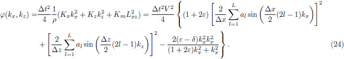
It’s very difficult to analyze the Eq.(23) and Eq.(24)directly, so we first analyze the dispersion relations oftwo FD schemes. Fig. 4 shows the dispersion curves for central-grid(Fig. 4a) and staggered-grid(Fig. 4b)FDschemes to approximate first-order derivative. Fig. 5 displays the specific numerical solutions of φ(k_x, k_z)withε = 0.3, δ = φ0.1 and L = 1. Fig. 4a indicates that using a central FD scheme to approximate the first-orderderivatives leads to numerical dispersion in the high wavenumber region and there exists singularity at theNyquist wavenumber, i.e., the FD response is near to zero at the Nyquist wavenumber. At the same time, L_xz > 0 and K_m < 0, then φ(k_x, k_z)< 0 as shown in Fig. 5a. This indicates that the central-grid hybrid PS/FDscheme for first-order P-wave equation is unstable for a model with anisotropic parameters ε > δ.

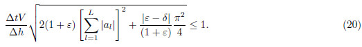
As shown in Fig. 4b, dispersion curves of staggered-grid FD scheme monotonically approach the theoreticalcurve with the increase of the order of finite difference scheme, i.e.,

So we only need to consider the case where L = 1. Since a₁ = 1, Eq.(24)reduces to

Inserting and into Eq.(26)yields

Using Eq.(21) and Eq.(27), we can obtain a stability condition concerning anisotropic parameters and spatialsampling step

For the special case Δx = Δz = Δh, the above stability condition can be further simplified to

The stability condition(29)reveals the limitation in application of the staggered-grid hybrid PS/FD schemefor first-order anisotropic pure P-wave equation. Clearly, compared with constraint condition ε ≥ δ thatAlkhalifah’s equation(2000) and other similar pseudo-acoustic equations(e.g. Zhou et al., 2006; Duveneck and Bakker, 2011; Zhang et al., 2011)require, the condition(29)is more easily to be satisfied, since mostsedimentary rocks have anisotropy in the weak-to-moderate range(i.e., < 0.2). In other words, pure P-waveequation extends the usefulness of acoustic anisotropy.

4 METHOD TO IMPROVE STABILITY

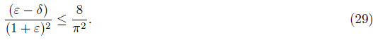
Figure 5a shows that the instability region is restricted to wavenumbers near Nyquist. So we can apply alow-pass filter to the wavenumber operators. Thus Eq.(6)can be rewritten as

where D[ ] denotes filtering.

We use conventional Z transform to construct the wavenumber-domain weighting function(Yan and Sava, 2009). For the case of second-order centered derivatives, the stencil has the following Z transform representation

Transforming form Z domain to the wavenumber domain, we obtain

which enables us to define the second-order weighting function:

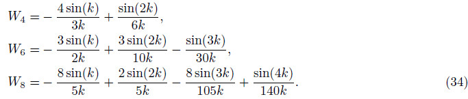
Here, the wavenumber k is normalized. Similarly, we can construct weights for fourth-, sixth-, and eighthorder weighting functions:

Figure 6 displays the filter functions applied to the wavenumber operators. The advantage of this low-passfilter is its flexibility. If the value of |ε - δ| is large, we choose the low-order filter functions, otherwise, we usehigh-order filter functions so as to preserve the high wavenumber contents.

5 NUMERICAL EXAMPLES

In this section, some synthetic examples are usedto validate the proposed algorithm. We first use homogeneous models with the vertical velocity V = 3000m·s^-1 to test pure P-wave Eq.(6) and compare it withanisotropic elastic equation and pseudo-acoustic equation(Duveneck et al., 2008)using an impulse response.The source wavelet for this example is Ricker waveletwith a peak frequency f_m=25 Hz located at middleof model. We use a 10 m grid space and a 1 mstime step size. Fig. 7 shows the vertical componentsin first homogeneous model with anisotropic parameters ε = 0.2, δ = -0.05, computed by anisotropicelasticequation(Fig. 7a), pseudo-acoustic equation(Fig. 7b), and pure P-wave equation using central-grid hybridPS/FD scheme(Fig. 7c and 7d) and staggered-grid hybrid PS/FD scheme(Fig. 7e). The difference betweenFig. 7c and 7d is that Fig. 7d is obtained by filtering the wavenumber operator with an eight-order filter functionin numerical implementation. From Fig. 7, we can clearly see that:(1)Pure P-wave equation is completely freefrom shear-wave compared with elastic wave equation and conventional pseudo-acoustic VTI equation;(2)Thehybrid PS/FD scheme on a central grid suffers from some numerical instabilities when the anisotropy parametersε > δ and low-pass filtering method significantly alleviate instability problem;(3)The staggered-grid hybridPS/FD scheme provides a stable pure P-wave propagator. The second example is still a homogeneous VTImodel but with anisotropic parameters ε = 0.05, δ = 0.2. Fig. 8 displays the stable wavefiled snapshots obtainedby anisotropic elastic equation(Fig. 8a) and pure P-wave equation using hybrid central-grid PS/FD scheme(Fig. 8b) and staggered-grid hybrid PS/FD scheme(Fig. 8c). These two examples testify our stability analysis. Both hybrid schemes are stable for VTI model with anisotropic parameters ε ≤ δ, but for the case ε > δ, thecentral-grid hybrid PS/FD scheme can’t provide stable numerical results.

Figure 9 displays direct comparison between elastic wave(solid black line) and pure P wave(dashed grayline)seismograms. The pure P-wave simulation result is practically same as that from the elastic equation inkinematic and dynamic respects, except that the latter is completely free from shear wave. But note that, theamplitude behavior of P-wave equation do not match that of the elastic equation for heterogeneous media sincepure P-wave can’t h and le the converted waves. Further investigation in this area remains to be a research topic.

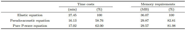
Next, we use a modified Hess VTI model(Fig. 10)with spatial variations in all model parameters to testthe robustness of the proposed method for complex anisotropic models. The model dimensions are nx = 1200 and nz = 750, with grid sampling step of 12.5 m in two directions. We again use the Ricker wavelet as the sourcewavelet with a peak frequency of 25 Hz. We put the source wavelet location at the position of(x, z)=(650, 50).The propagation time step is 1 ms. Fig. 11 shows the wavefield snapshots computed by(a)elastic equation and (b)first-order pure P-wave equation using staggered-grid hybrid PS/FD scheme. Fig. 12 is the correspondingcommon-source gathers. From the snapshots and gathers, we can see that even in such complex anisotropicmodel with sharp contrasts, first-order pure P-wave equation can also provide stable and accurate numericalresults. Table 1 shows the average time costs and memory requirements of three different equations. The twoacoustic approximation equations are close in computational costs and both more efficient than original elasticequation. In fact, the pure P-wave equation can use larger spatial sampling step since it doesn’t need to considerthe numerical dispersion caused by shear wave. Thus it can be more efficient further.

6 CONCLUSIONS

Starting from the VTI exact phase velocity, the first-order pure P-wave equation is derived by using afirst-order Taylor series expansion to the radical. We adopt an efficient hybrid PS/FD scheme to solve the pureP-wave equation rather than using PS method alone. The stability condition of such scheme on central and staggered grids is investigated. Stability analysis shows that the hybrid scheme on a staggered grid is morestable than that on a central grid. To deal with the instability problem of the central-grid hybrid PS/FDscheme, we apply a low-pass filter to wavenumber operator. The kinetic and dynamic accuracy of the proposedequation is analyzed by comparison with original elastic equation and pseudo-acoustic equation. Synthetic2D examples demonstrate that the proposed first-order pure P-wave equation provides stable and kineticallyaccurate numerical results. In spite of its dynamic inaccuracy in heterogeneous media, the first-order pure Pwave equation is practically promising in anisotropic modeling and migration algorithms oriented to subsurfacestructures.

ACKNOWLEDGMENTS

This work was supported by the National Natural Science Foundation of China(41174100), Large-scaleOil & GasField and Coalbed Methane Development Major Projects(2011ZX05019-008-08), and China NationalPetroleum Corporation(2014A-3609). We are also grateful to the reviewers and the editor for their very detailed and constructive comments that significantly improve the original manuscript. We thank Professor ShuTingWang, Doctor Gang Fang and Dong Han for their useful suggestions. We would like to thank Hess for makingthe VTI model available.

Appendix The Relation Between Two Different Acoustic Approximations

In this appendix, we briefly discuss the relation between pseudo-acoustic equation and pure P-wave equation. The dispersion relation that Alkhalifah(2000)presented is as follows

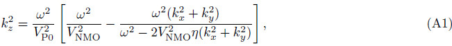
where V_P0 ² is P-wave vertical velocity along the symmetry axis, ω is angular frequency, isthe small offset P-wave normal moveout velocity, η =(ε - δ)/(1 + 2δ)is effective anisotropy parameter, k_x, k_y and k_z are spatial wavenumbers in x, y and z directions, respectively. After some algebraic manipulations, Eq.(A1)can be cast into the equivalent rational fractional form:

The approximate 3D dispersion relation governing pure P wave is

Comparing two dispersion relations(A2) and (A3), we can find there exists the following elliptic approximationin the denominator of fractional(anelliptic)term,

This indicates that pure P-wave dispersion relation obtained by first-order Taylor expansion is a further ellipticapproximation for acoustic assumption. These are of course not the only possible pure P-wave approximations.Further approximations could be derived by various other modifications of the fractional(anelliptic)terms.One could also potentially gain greater accuracy by retaining higher order terms in a Taylor, Pad′e, or similarexpansion to replace the square root of Eq.(2).