 2015, Vol. 58


2. University of Chinese Academy of Sciences, Beijing 100049, China
With the increase of exploration depth of oil-producing region, there are increasing needs for the higher precision imaging and inversion, and then as a basis of imaging and inversion methods, numerical modeling technology becomes more and more important. Numerical modeling method based on wave equation contains the kinematics and dynamics characteristics of wavefields, and is widely used(Cheng et al., 2008). The finitedifference method(Alterman and Karal, 1968; Kelly et al., 1976; Dablain, 1986; Igel et al., 1995) and pseudospectral method(Gazdag, 1981; Kosloff and Baysal, 1982; Carcione, 1992)as two numerical modeling method based on wave equation are well known. The finite-difference method was put forward in the late 1960s, Alterman and Karal(1968)first used explicit 2nd order finite-difference operator to simulate the elastic wavefields in layered media. Kelly et al.(1976)proposed the finite-difference method which was suitable for heterogeneous media. Dablain(1986)carried out scalar wave numerical modeling using high-order operators. Liu et al.(1998)derived the finite-difference operators of any even-order accuracy for any even derivative from the Taylor series expansion. Dong et al.(2000)derived a staggered-grid high-order finite-difference method for first-order elastic wave equation. Pei and Mou(2003)derived staggered-grid finite-difference operators of any even-order accuracy. Liu and Sen(2009a, 2010)proposed a new time-space domain high-order finite-difference method for the acoustic wave equation, and then Yan and Liu(2013a, 2013b)extended their methods to visco-acoustic and anisotropic acoustic equation.
Numerical dispersion of the finite-difference method is inevitable because of the approximation of difference operator to differential operator. In order to decrease the numerical dispersion, we have to adopt a finer grid or lower wavelet frequency, however, which will respectively bring huge computational cost and the loss of part of the high frequencies. Some geophysicists have proposed a variety of methods to suppress the numerical dispersion. The first method is FCT technology. Boris and Book(1973)first applied the FCT in reducing the numerical dispersion. Yang and Teng(1997)extended this method to three-component seismic numerical modeling for anisotropic media. The second method is optimization methods. Holberg(1987) and Robertsson(1994)minimized the error using optimization methods to calculate the finite-difference coefficients. Zhang and Yao(2012)used the simulated annealing algorithm to minimize the objective functions constructed by the maximum norm to get the finite-difference coefficients, which has larger wave number coverage and smaller margin of error. Liu(2013)adopted least-squares method to get global optimized finite-difference operators. Yang et al.(2014)extended this method to staggered-grid finite-difference methods. The third method is truncated windows methods. The methods are based on the knowledge that the pseudo-spectral method can be interpreted as the limit of finite-difference schemes of increasing orders(Fornberg, 1987). Zhou and Greenhalgh(1992)chose the generalized powered Hanning window to get optimized finite-difference operators. Igel et al.(1995)used Gaussian window to develop staggered-grid finite-difference operators. Chu and Stoffa(2012)unified the finite-difference method and the pseudo-spectral method using the binomial window, and adopted an improved binomial window to get optimized finite-difference operators, and they thought that this strategy of improved binomial window is the same as that of truncated finite-difference methods proposed by Liu and Sen(2009b)in essence.
In space domain, we can truncate the spatial convolution series of the pseudo-spectral method to get finitedifference method. In terms of digital signal processor, truncating is equal to using a window function which will cause spectrum leakage. In order to suppress the numerical dispersion, choosing some suitable window function is necessary, different window functions have different results. Specifically, the window function which has narrower main lobe and larger attenuation of side lobe in its amplitude response bring higher accuracy of finite-difference approximation, in this paper, we design a window function based on this theory to truncate the spatial convolution series of the pseudo-spectral method to get optimized finite-difference operators which can efficiently suppress the numerical dispersion.
The generalized weighted Hanning window designed by Zhou and Greenhalgh(1992)is one of trigonometric window functions, which has relatively small attenuation of side lobe in amplitude response thus leads to the fluctuation of accuracy error. The fluctuation of accuracy error greatly affects the result of numerical modelling(Zhang and Yao, 2012). The improved binomial window proposed by Chu and Stoffa(2012)has a wide main lobe in its amplitude response, resulting in a narrow wave number coverage range, at the same time, the accuracy error curves of finite-difference operators based on improved binomial window show obvious fluctuation especially for the low-order operators(below twelfth-order). In this paper, we first analyze the influence on the accuracy of finite-difference operators caused by the properties of main lobe and side lobe in the amplitude response of truncated windows, and then introduce the auto-convolution and weighted combination to the design of window functions. Finally, we design Chebyshev auto-convolution combined window which has narrow main lobe and large attenuation of side lobe in its amplitude response. Through adjusting three parameters of auto-convolution combined window, visually and straight forwardly control the properties of main lobe and side lobe to adjust the accuracy of finite-difference approximation.
2 APPROXIMATION ERROR ANALYSIS 2.1 Conventional Finite-Difference OperatorsAccording to the discrete signal sampling theorem, a b and limited continuous signal f(x)can be reconstructed by a uniform sampling signal fn using the sinc interpolator(Diniz et al., 2012):
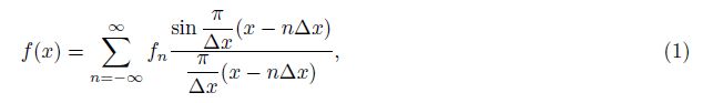
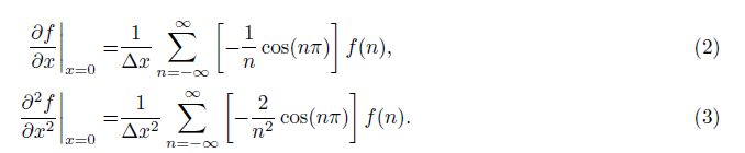
We separately compute the first derivative and the second derivative at x = 0 by differentiating both sides of Eq.(1):
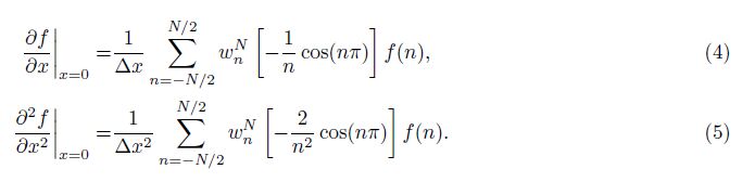
Zhou and Greenhalgh(1992)designed the generalized weighted Hanning window which is one of trigonometric window functions. Igel et al.(1995)used Gaussian window. Chu and Stoffa(2012)proposed the improved binomial window. We compare these four window functions, analyze the influence on the accuracy of finitedifference operators caused by the properties of main lobe and side lobe in the amplitude response of window functions.
Figure 1 and Fig. 2 respectively display these four window functions for N = 24 and their amplitude responses. As shown in Fig. 1 and Fig. 2, the improved binomial window applies more tapering than other windows, accordingly, has wider main lobe in its amplitude response. Diniz et al.(2012)thought that wide main lobe means wide transition b and which reduces the wavenumber coverage and causes numerical dispersion for the part of high wavenumber. Compared with other windows, the improved binomial window has widest main lobe, as a result, the finite-difference operators truncated by the improved binomial window are not accurate for the part of high wavenumber, meanwhile, the improved binomial window has largest attenuation of side lobe, which bring best stability of accuracy error. As for Kaiser and Chebyshev window functions, we can adjust the parameters β and r which are respectively the parameters of these two window functions to get different amplitude responses. Here, we set r = 60 and β = 5.

|
Fig.1 Comparison of window functions, N = 24 |

|
Fig.2 Amplitude response of four window functions, frequency points M = 512 |
Figure 3 shows the amplitude responses of Kaiser window function(β = 2, 5, 9) and Chebyshev window function(r = 35, 60, 95)for N = 24.

|
Fig.3 Amplitude response of two window functions, different β and r, frequency points M = 512 (a)Kaiser window;(b)Chebyshev window. |
As demonstrated in Fig. 3, for Kaiser window function, with the increase of β, main lobe becomes wider and attenuation of side lobe becomes larger; for Chebyshev window function, with the increase of r, the variation is the same. Compared with these two window functions, Chebyshev window function has relatively larger attenuation of side lobe, and the finite-difference operators truncated by Chebyshev window function have better stability of accuracy error.
n = 0 is singular point. Lee and Seo(2002)think that Eq.(2) and Eq.(3)can be expressed as follows:
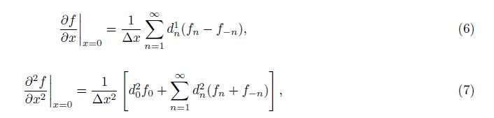
We can get finite-difference operators by truncating Eqs.(6) and (7)using window functions, which can be generalized to the Eqs.(8) and (9):
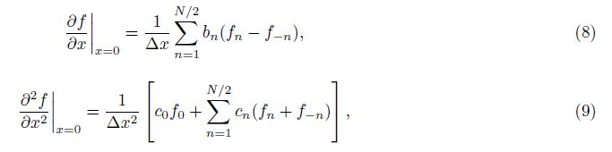
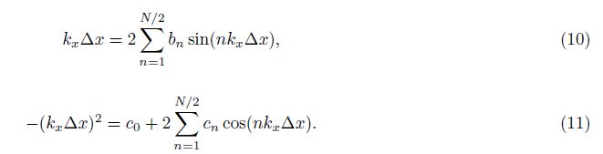
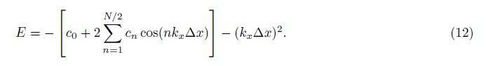
Figure 4a shows that, accuracy error curves for second derivative of Hanning and Kaiser window functions have wider wavenumber coverage. The improved binomial window brings the narrowest wavenumber coverage. The finite-difference operators truncated by Chebyshev window function has appropriate wave number coverage. We magnify the accuracy error curves one thous and times; the fluctuation of accuracy error curves of Kaiser and Hanning windows is more obvious than that of the remaining two windows. Considering the wave number coverage and the fluctuation of accuracy error curves, Chebyshev window is a better choice to truncate Eqs.(6) and (7)to derive optimized finite-difference operators for elastic wave modelling.

|
Fig.4 Accuracy error for second derivative of four window truncated finite-difference operators(N = 24) (a)Accuracy error;(b)Magnified 1000 times. |
We apply one auto-convolution on an(N + 1)-point Chebyshev window function to get an(2N + 1)-point Chebyshev auto-convolution window function, N is an even number. Similarly, we can perform L autoconvolutions on Chebyshev window function to get L-order Chebyshev auto-convolution window function. We first perform the Fourier transform on Chebyshev window function, ω = kx△x, which gives

Amplitude responses of Chebyshev auto-convolution window functions after different number of autoconvolutions are shown in Fig. 5. Auto-convolutions obviously increase the attenuation of side lobe and make the main lobe wider at the same time, with the increase of number of auto-convolutions, the impact is greater.

|
Fig.5 Amplitude response of Chebyshev auto-convolution window function(N = 4)L=1, 2, 3, 4, 5, 6 |
We fix the length of window functions, here N = 24. Two and four auto-convolutions are separately flagged as L = 2 and L = 4. The amplitude responses of Chebyshev auto-convolution window functions after two and four auto-convolutions are shown in Fig. 6, with the increase of number of auto-convolutions, main lobe becomes wider and attenuation of side lobe larger.

|
Fig.6 Amplitude response of Chebyshev auto-convolution window function(Fix N = 24), L=2, 4 |
We still utilize the Eq.(12)to measure the accuracy errors of the finite-difference operators for the second derivative. Fig. 7 displays the accuracy error curves of the finite-difference operators truncated by three window functions shown in Fig. 6 for N = 24.

|
Fig.7 Accuracy error for second derivative of auto-convolution window truncated finite-difference operators(N = 24) (a)Accuracy error;(b)Magnified 1000 times. |
As shown in Fig. 7, with the increase of the number of auto-convolutions, the finite-difference operators truncated by the auto-convolution window functions have narrower wavenumber coverage, however, have better stability of accuracy error. Considering the wavenumber coverage and stability of accuracy error, we can get window function which has good properties of truncation through performing two auto-convolutions.
Based on the previous analysis, our purpose is to design a window function which has narrow main lobe and large attenuation of side lobe, and get the finite-difference operators which have better stability of accuracy error on the premise of maintaining appropriate wave number coverage, thus we introduce a linear weighted function:

We can choose different auto-convolution combined window functions through adjusting three parameters to get the optimized finite-difference operators. The parameters are ripple rate r, the number of autoconvolutions L and weight coefficient λ. In this paper, we set λ = 0.89, r = 60, L = 2. Fig. 8 displays the accuracy error curves of the finite-difference operators(N=8, 12, 16, 24)truncated by the Chebyshev auto-convolution combined window function for the second derivative. The finite-difference operators based on Chebyshev autoconvolution combined window have much higher accuracy than the conventional finite-difference operators. The accuracy of our optimized eighth-order and twelfth-order finite-difference operators can respectively reach, even exceed that of the conventional twelfth-order and twenty-fourth-order finite-difference operators. The maximum deviation of absolute accuracy error curves is within a range of [0, 0.0004].

|
Fig.8 Accuracy error for second derivative of the operators based on Chebyshev auto-convolution combined window function for different N(different orders) (a)Accuracy error;(b)Magnified 1000 times. |
Figure 9 displays the comparison between the finite-difference operators based on the improved binomial window and the operators based on Chebyshev auto-convolution combined window function. As see from Fig. 9, apparently, for low-order operators(especially eighth-order in Fig. 9), the accuracy error curve of the operator based on the improved binomial window has obvious fluctuation, and for high-order operators, in the condition of same order, the accuracy of operators based on the improved binomial window is lower than that of the operators based on Chebyshev auto-convolution combined window function.

|
Fig.9 Comparison of accuracy error for second derivative between the operators based on Chebyshev autoconvolution combined window function and improved binomial window for different N(different orders) (a)Accuracy error;(b)Magnified 1000 times. |
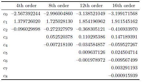
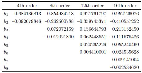
Finite-difference weights truncated by the Chebyshev auto-convolution combined window function for the second derivative with N=4, 8, 12, 16 are given in Table 1.
| Table 1 Chebyshev auto-convolution window truncated finite-difference operator coefficients for the second derivative |
Similarly, we also use Eq.(12)to measure the accuracy errors of the finite-difference operators for the first derivative:
Figure 10 displays the accuracy error curves of the finite-difference operators(N=8, 12, 16, 24)truncated by the Chebyshev auto-convolution combined window function for the first derivative. As shown in Fig. 10, compared with the conventional finite-difference operators, the finite-difference operators based on Chebyshev auto-convolution combined window function have wider wavenumber coverage and better statability of accuracy error for the same order.

|
Fig.10 Accuracy error for first derivative of the operators based on Chebyshev auto-convolution combined window function for different N(different orders) (a)Accuracy error;(b)Magnified 1000 times. |
Finite-difference weights truncated by the Chebyshev auto-convolution combined window function for the first derivative with N=4, 8, 12, 16 are given in Table 2.
| Table 2 Chebyshev auto-convolution window truncated finite-difference operator coefficients for the first derivative |
The linear theory of elasticity establishes a relationship between vector wavefield displacement and the dimensionless linear strain tensor:

The linear strain tensor εkl can be related to the stress tensor σij using a constitutive relationship:

Substituting Eqs.(16) and (17)into the equations of motion derived from Newton’s second law, that describe wave propagation for anisotropic elastic media, ignoring the body force per unit volume:

A 2D homogeneous medium is defined on a grid of 255×300 with grid spacing of 5 m. The P-wave velocity is 2000 m·s-1, The S-wave velocity is 1500 m·s-1, a point source is located at the center of the media. Fig. 11 displays the snapshots of impulse responses generated by the finite-difference operators(N=8)truncated by the Chebyshev auto-convolution combined window function and the conventional finite-difference operators(N=8, 12)at nt=500, the dominant frequency of a Ricker wavelet is 30 Hz.

|
Fig.11 Comparison of snapshot of impulse responses before and after using the operators based on Chebyshev auto-convolution combined window function(250 ms) (a)Using the 8th conventional operator(left is X component, right is Z component);(b)Using the 8th optimized operator(left is X component, right is Z component);(c)Using the 12th conventional operator(left is X component, right is Z component). |
Figure 11a is the snapshots(X and Z components)generated by the eighth-order conventional operator, which have obvious numerical dispersion. The eighth-order operator based on Chebshev auto-convolution combined window function can effectively suppress numerical dispersion as shown in Fig. 11b. Using the twelfthorder conventional operator can also significantly suppresses the dispersions(Fig. 11c)but it doubles the computational cost. In conclusion, Compared with the conventional eighth-order and twelfth-order finite-difference operators, our optimized eighth-order finite-difference operator based on Chebyshev auto-convolution combined window function has a better result.
3.2 Marmousi ModelTo further examine the quality of our optimized finite-difference operators based on combined window, we test on a Marmousi model. The grid is 737×750, △x=12.5 m, △z=4 m, the Marmousi P-wave velocity model is shown in Fig. 12, the S-wave velocity is a scaled version of the P-wave velocity with vS = vP/$\sqrt{3}$, the density is 1000 kg·m-3, the dominant frequency of a Ricker wavelet is 30 Hz, positioned at x=231.25 m, z=25 m. The record-length is 5 s with a time step of 0.0005 s.

|
Fig.12 This is the Marmousi P-wave velocity model |
We ran the code on a PC with a Intel(R)Core i5 2300 @2.8GHz CPU and a 192-core NVIDIA GTX550Ti GPU card. The version of CUDA is 4.2. We position the source at x=0.0 m, 2303.1 m, 4606.3 m, 6909.4 m, 9212.5 m.
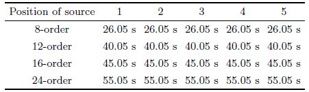
Computation cost using the conventional finite-difference operators and the finite-difference operators based on Chebyshev auto-convolution window function for different orders are given in Table 3 and Table 4.
| Table 3 Comparison of computation cost using the finite-difference operators based on Chebyshev auto-convolution window function for different orders |
| Table 4 Comparison of computation cost using the conventional finite-difference operators for different orders |
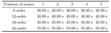
Figure 13 shows the comparison of a shot record for the Marmousi model computed by the conventional finite-difference operators(N=8, 12) and the finite-difference operators based on Chebyshev auto-convolution combined window function(N=8)(Z component). Figs. 13(b, c, d)is separately the zoomed in view of block 1, 2, 3 of Fig. 13a.

|
Fig.13 Comparison of a shot record for the Marmousi model computed by the conventional finite-difference operators and the finite-difference operators based on Chebyshev auto-convolution combined window function(Z component) (a)One shot record(left using the 8th conventional operator, middle using the 8th optimized operator, right using the 12th conventional operator);(b)Zoomed in view of a shot record(Block 1);(c)Zoomed in view of a shot record(Block 2);(d)Zoomed in view of a shot record(Block 3). |
The left figures of Figs. 13(b, c, d)generated by the eighth-order conventional operator have obvious numerical dispersion, and the middle figures of Figs. 13(b, c, d)generated by the eighth-order operators based on Chebshev auto-convolution combined window function have a better result, significantly suppress the dispersion. Using the twelfth-order conventional operator can also effectively suppresses the numerical dispersion(the right figures of Figs. 13(b, c, d)), however, compared with the shot record generated by the eighth-order operators based on Chebshev auto-convolution combined window function, it still has relatively obvious dispersion and doubles the computational cost. The numerical modelling results in the complex medium show that, the accuracy of the finite-difference operators based on Chebshev auto-convolution combined window function is better than that of the conventional finite-difference operators.
4 CONCLUSIONWe propose optimized finite-difference operators based on Chebyshev auto-convolution combined window function. We first analyze the influence on the accuracy of finite-difference approximation caused by the properties of amplitude responses of window function, narrower main lobe and larger attenuation of side lobe bring higher accuracy of finite-difference approximation, and significantly suppress numerical dispersion. Compared with the generalized powered Hanning window and improved binomial window, the Chebyshev auto-convolution combined window has better attributes of amplitude response to get optimized finite-difference operators, and can visually and more intuitively adjust the accuracy of finite-difference approximation through adjusting three parameters.
The finite-difference operators based on Chebyshev auto-convolution combined window have higher accuracy than that of the conventional finite-difference operators. In this paper, we set λ=0.89, r=60, L=2. The eighth-order and twelfth-order operators based on Chebyshev auto-convolution combined window can respectively reach, even exceed the accuracy of the twelfth-order and twenty-fourth-order conventional finite-difference operators, and the maximum deviation of absolute error is within [0, 0.0004]. For higher-order operators, the accuracy increase becomes more obvious. Numerical dispersion analysis and elastic wave numerical modelling demonstrate that our finite-difference operators have higher accuracy than the conventional finite-difference operators and can more efficiently suppress numerical dispersion under the same condition.
ACKNOWLEDGMENTSWe would like to thank the two anonymous reviewers for their careful reading and valuable comments on the manuscript. This work was supported by the National Natural Science Foundation of China(41174047, 40874024 and 41204041).
| [1] | Alterman Z,Karal F C Jr.1968.Propagation of elastic waves in layered media by finite difference methods.Bulletin of Seismological Society of America,58(1):367-398. |
| [2] | Boris J P,Book D L.1973.Flux-corrected transport.I.SHASTA,a fluid transport algorithm that works.Journal of Computational Physics,11(1):38-69. |
| [3] | Carcione J M,Kosloff D,Behle A,et al.1992.A spectral scheme for wave propagation simulation in 3-D elastic-anisotropic media.Geophysics,57(12):1593-1607,doi:10.1190/1.1443227. |
| [4] | Cheng B J,Li X F,Long G H.2008.Seismic waves modeling by convolutional Forsyte polynomial differentiator method. |
| [5] | Chinese J.Geophys.(in Chinese),51(2):531-537. |
| [6] | Chu C L,Stoffa P L.2012.Determination of finite-difference weights using scaled binomial windows.Geophysics,77(3):W17-W26,doi:10.1190/GEO2011-0336.1. |
| [7] | Dablain M A.1986.The application of high-order differencing to the scalar wave equation.Geophysics,51(1):54-66,doi:10.1190/1.1442040. |
| [8] | Diniz P S R,da Silva E A B,Netto S L.2012.Digital Signal Processing System Analysis and Design.Beijing:China Machine Press. |
| [9] | Dong L G,Ma Z T,Cao J Z,et al.2000.A staggered-grid high-order difference method of one-order elastic wave equation.Chinese J.Geophys.(in Chinese),43(3):411-419. |
| [10] | Fornberg B.1987.The pseudospectral method:Comparisons with finite differences for the elastic wave equation.Geophysics,52(4):483-501,doi:10.1190/1.1442319. |
| [11] | Gazdag J.1981.Modeling of the acoustic wave equation with transform methods.Geophysics,46(6):854-859,doi:10.1190/1.1441223. |
| [12] | Holberg O.1987.Computational aspects of the choice of operator and sampling interval for numerical differentiation in large-scale simulation of wave phenomena.Geophysical Prospecting,35(6):629-655,doi:10.1111/j.1365-2478.1987.tb00841.x. |
| [13] | Igel H,Mora P,Riollet B.1995.Anisotropic wave propagation through finite-difference grids.Geophysics,60(4):1203-1216,doi:10.1190/1.1443849. |
| [14] | Kelly K R,Ward R W,Treitel S,et al.1976.Synthetic seismograms:A finite-difference approach.Geophysics,41(1):2-27,doi:10.1190/1.1440605. |
| [15] | Kosloff D D,Baysal E.1982.Forward modeling by a Fourier method.Geophysics,47(10):1402-1412,doi:10.1190/1.1441288. |
| [16] | Lee C,Seo Y.2002.A new compact spectral scheme for turbulence simulations.Journal of Computational Physics,183(2):438-469,doi:10.1006/jcph.2002.7201. |
| [17] | Liu Y,Li C C,Mou Y G.1998.Finite-difference numerical modeling of any even-order accuracy.OGP(in Chinese),33(1):1-10. |
| [18] | Liu Y,Sen M K.2009a.A new time-space domain high-order finite-different method for the acoustic wave equation.Journal of Computational Physics,228(23):8779-8806,doi:10.1016/j.jcp.2009.08.027. |
| [19] | Liu Y,Sen M K.2009b.Numerical modeling of wave equation by a truncated high-order finite-difference method.Earthquake Science,22(2):205-213,doi:10.1007/s11589-009-0205-0. |
| [20] | Liu Y,Sen M K.2010.Acoustic VTI modeling with a time-spacedomain dispersion-relation-based finite-difference scheme.Geophysics,75(3):A11-A17,doi:10.1190/1.3374477. |
| [21] | Liu Y.2013.Globally optimal finite-difference schemes based on least squares.Geophysics,78(4):T113-T132,doi:10.1190/geo2012-0480.1. |
| [22] | Pei Z L,Mou L G.2003.A staggered-grid high-order difference method for modeling seismic wave propagation in inhomogeneous media.Journal of China University of Petroleum(Edition of Natural Science)(in Chinese),27(6):17-27. |
| [23] | Robertsson J O A,Blanch J O,Symes W W,et al.1994.Galerkin-wavelet modeling of wave propagation:Optimal finitedifference stencil design.Mathematical and Computer Modelling,19(1):31-38,doi:10.1016/0895-7177(94)90113-9. |
| [24] | Yan H Y,Liu Y.2013a.Visco-acoustic prestack reverse-time migration based on the time-space domain adaptive highorder finite-difference method.Geophysical Prospecting,61(5):941-954,doi:10.1111/1365-2478.12046. |
| [25] | Yan H Y,Liu Y.2013b.Pre-stack reverse-time migration based on the time-space domain adaptive high-order finitedifference method in acoustic VTI medium.Journal of Geophysics and Engineering,10(1):015010,doi:10.1088/1742-2132/10/1/015010. |
| [26] | Yang D H,Teng J W.1997.FCT finite difference modeling of three-component seismic records in anisotropic medium.OGP(in Chinese),32(2):181-190. |
| [27] | Yang L,Yan H Y,Liu H.2014.Least squares staggered-grid finite-difference for elastic wave modelling.Exploration Geophysics,45(4):255-260,doi:10.1071/EG13087. |
| [28] | Zhang J H,Yao Z X.2013.Optimized finite-difference operator for broadband seismic wave modeling.Geophysics,78(1):A13-A18,doi:10.1190/GEO2012-0277.1. |
| [29] | Zhou B,Greenhalgh S A.1992.Seismic scalar wave equation modeling by a convolutional differentiator.Bulletin of the Seismological Society of America,82(1):289-303. |