1 INTRODUCTION

Regional geophysics aims to obtain information about the structures of the crust and upper mantle by applying advanced observation technologies to detect geophysical fields. The geophysical observations are carried out with some prescriptive grids to reveal the three-dimensional structures and tectonic patterns of the lithosphere, finally providing scientific knowledge for resources exploration, reducing geological hazards and keeping ecological equilibration. The observation grids can uniformly cover the whole region with fine meshes, overcoming the geological limitation of observation related to rock outcrops or boreholes. In particular, it contains information comprehensively coming from the source bodies in different depths, which enables us to infer the three-dimensional structures and tectonic patterns of the lithosphere, on the basis of physical laws. For these reasons, regional geophysics has been attracting increasing attentions.

Geophysical fields comprise gravity and magnetic field, reflection seismic wave field, and geothermal field. Geophysical observations can be carried out on the ground, by airborne or by artificial-satellites. The gravity field decays with the distance between the observation station and the source, which can exist in the lower crust. And the cost for regional gravity investigation is low and acceptable. Furthermore, China has almost completed regional ground gravity surveys with scale of 1:220150104, and the satellite gravity data are available for its surrounding areas. Therefore, applying the regional gravity data to reveal three-dimensional density structures and tectonic patterns becomes reality to our regional geophysical studies. However, in order to reveal three-dimensional density structures and tectonic patterns, we have to develop more advanced data processing methods.

After years of researches, we have developed multi-scale wavelet analysis, spectral analysis of potential fields, geophysical inversions, and scratch recognition methods in regional gravity data processing. These methods have different functions and can be combined to a new data processing system, comprising four modules that are spectral analysis for defining the equivalent density layers and estimating depth of the layers, decomposition of the gravity field by using the multi-scale wavelet analysis, density distribution inversion of the decomposed gravity anomalies, and the scratch analysis for locating deformation belts, referring to Fig. 1. This data processing system is called as the multi-scale scratch analysis. We will briefly introduce its basic principles and application results in this paper.

2 SCALE-DEPTH CONVERSION LAW OF THE MULTI-SCALE ANALYSIS FOR BOUGUER GRAVITY FIELD

Since 1990, we have conducted researches on multi-scale wavelet analysis of gravity field, producing positive results for the field decomposition. Following the Mallat's Pyramidal algorithm(Mallat, 1989; Daubechies, 1990), we have constructed a new wavelet base especially for decomposition of the regional gravity field(Hou and Yang, 1997; Hou et al., 1998). As our previous papers show the details of the theory of two-dimensional discrete wavelet transformation and its application to regional gravity-field decomposition(Hou and Yang, 1997; Hou et al., 1998; Yang et al., 2001; Hou and Yang, 2011; Hou and Yang 2012), we do not need to repeat them in this paper. Regional gravity field can be expressed as two-dimensional single-valued function, while the crustal three-dimensional density model can be represented as three-dimensional single-valued function. If without additional constraint laws, we cannot obtain the three-dimensional density structural model only based on the two-dimensional surface observation data. The additional law is called the scale-depth conversion law for the wavelet transform of the Bouguer gravity field, which is derived as follows.

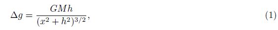
The basis of the multi-scale wavelet analysis for regional gravity data processing is that the horizontal scale of gravity anomalies is proportional to the buried depth of the gravity sources. In other words, the deeper the source buries, the larger the horizontal scale of the anomaly becomes. For instance, the gravity anomaly of a sphere object can be written as(Zeng, 2005)

where G is the gravitational constant, M is the mass of the sphere, h is the depth of the sphere center, and x is the horizontal distance from observed points to the projection of the sphere center on the observation plane. Define the horizontal width of gravity anomaly W satisfying W = 2x', in which x' is the horizontal distance between the origin to the point where the maximum anomalous values attenuates to the half. Then W also represents characteristic scale of the isolated anomaly. Substituting x' into Eq.(1)yields Thus, the deeper the burial depth h of field source is, the larger the horizontal scale W of the anomaly becomes. The burial depth and the horizontal scale are approximately proportional to each other. Nevertheless, due to the different shapes of buried sources, the scaling factor α may vary with source shapes, satisfying the condition α = 0.2 ~ 0.9. For instance, the value of α can be chosen as 0.8 for intrusive thin dykes.

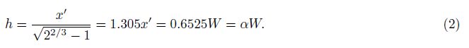
When the gravity anomalies are produced by the superposition of several field sources, they will no longer have similar characteristic scales from Eq.(2). Specifically, the characteristic scale W for the spherical source with the center depth of 4 km in upper crust is 6.13, and that with the center depth of 34 km in lower crust is 52.1. However, the scale may range from 6 km to 52 km when the above two anomalies are added together, indicating no characteristic scale after the superposition. The multi-scale wavelet analysis utilizes the characteristic scale of the desired wavelet base to recover the characteristic scale in the ground superimposed anomalies, and decomposes them with different scales, making the decomposed wavelet details obtain characteristic scales again. For the above example, the superimposed anomalies are decomposed by the wavelet analysis with the wavelet scale of 6 km, 12 km, 24 km and 48 km. The first-order wavelet detail D₁ with the scale of 6 km extracts the anomaly field produced by the spherical source buried with the center depth of 4 km in upper crust. The fourth-order wavelet detail D₄ with the wavelet scale of 48 km draws the anomaly produced by the spherical source buried with the center depth of 34 km in lower crust. In a certain sense, the wavelet details can restore the characteristic scale in gravity field. Therefore, the multi-scale wavelet analysis can be an important technology for delineating three-dimensional crustal density structures.

Assume the gravity data spacing in a uniform square grid as △. When applying the conventional wavelet multi-scale analysis, the wavelet base will take 4 sampling points(Mallat, 1989), with the shape of peaks and valleys and the characteristic scale of about half of the peak width, namely △/2. The scale of the wavelet details increases with the power of 2 during wavelet transforms. Defining the order of the wavelet details as n, the characteristic scale of n-order wavelet details can be written as

The multi-scale wavelet analysis requires that the characteristic scale L_n of wavelet details should match with the scale W of the gravity anomalies. Substituting Eq.(3)into Eq.(2), gives and Eq.(5)represents the relation between the burial depth h of field sources and the nth-order wavelet details, namely the scale-depth conversion law in the multiscale wavelet analysis for decomposition of Bouguer gravity field. For some ground gravity data sets with different observation meshes or survey scales, the characteristic scales of wavelet details are estimated by Eq.(3) and listed in Table 1. The gravity data sets with the sampling spacing greater than 20 km cannot be suitable for multi-scale wavelet analysis and three-dimensional characterization of fine crustal density structures(underlined numbers in Table 1). While if the sampling spacing is less than 1 km, it can be good only for decomposition the density disturbance of the upper crust because of too small scale of wavelet details.

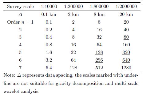
In summary, the greater the depth of field sources is, the larger the horizontal scale of ground gravity anomalies, as well as the density disturbance becomes. So after multi-scale wavelet decomposition of gravity data, small-scale wavelet details indicate density distribution of shallow sources, whereas large-scale wavelet details represent the distribution of deep sources. Since we presented multi-scale wavelet analysis for gravity data processing, the method has already showed good results(Hou et al., 1997, 1998, 2011; Yang et al., 2001). The reason for that is wavelet details reflect sources distribution in different burial depths, which can be applied to reveal crustal three-dimensional density disturbances.

3 DEPTH EQUATION FOR THE EQUIVALENT LAYERS OF WAVELET DETAILS

Regional gravity can be regarded as a two-dimensional single-valued function △g(x, y). After multi-scale wavelet decomposition, the wavelet details are sampling datasets of three-dimensional single-valued function △D(x, y, n). But crustal three-dimensional density model can be expressed as the function of the burial depths of density disturbance sources. We must add an additional constraint law to transform the wavelet details △D(x, y, n)to sampling datasets of △D(x, y, h), and then obtain gravity anomaly datasets corresponding to source equivalent layers at different depths. Ideally, we expect to decompose the regional field into four subanomalies correlated to the upper, middle and lower crust, and the relief on the top of the upper mantle. In fact, theory for interpretation of potential field in the frequency domain has provided basis for solving this problem. And to potential field, the frequency and wave-number domain are synonymous, referring to the frequency of the anomaly varying with the distance.

The frequency-domain theory of potential fields has demonstrated that for a single gravity source body, the slope of logarithmic power spectrum of its gravity anomaly is proportional to the burial depth of the source body; whereas for multiple source bodies, it will be proportional to the average depth of sources(Bhimasankakam et al., 1977; Yang et al., 1978; Yang et al., 1979; Yang 1979, 1985, 1986a, 1986b). In the case of horizontal cylinder, the logarithmic power spectrum is L_nS(ω)= -L_n(2π²Gr²ρ)ωh, in which G is gravitational constant; ρ is the density difference between the source body and its surrounding rock; ω is the circular frequency; r is the radius; h is the burial depth. The logarithmic power spectrum is inversely proportional to the frequency(wave number), and the proportional coefficient β is L_n(2π²Gr²ρ). For multiple source bodies, it will be proportional to the average depth of sources. Therefore, the recognizable straight segments with different dipping slopes in the spectral curves indicate depths of different equivalent layers of density disturbance. The steeper the straight segment is, the deeper the sources are buried. In other words, if there exist a certain amount of recognizable linesegments with different slopes, then we can decompose the regional gravity field into sub-anomalous sets. These sub-anomalous datasets are the wavelet details or the detail combinations of the regional gravity, corresponding to different source equivalent strata at different depths. Thus, depths of equivalent layers can be approximately expressed as

where hn is the depth of equivalent source layer correlated to the n-order wavelet detail; △S/△F is the maximum slope of the spectrum; β is the proportional coefficient, which may vary with source shapes.

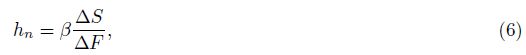
After achieving N sub-anomalies by combining the wavelet details, we perform two-dimensional Fourier transform of each sub-anomaly to find its power spectrum, which is the average power spectrum curve of every direction. From Eq.(6), we can calculate the burial depths of the equivalent layers correlated to different subanomalies, and then transform the wavelet details △D(x, y, n)to sampling datasets of △D(x, y, h). It should be noted that decomposing regional gravity field depends on the spectral properties of regional gravity field, but by no means that all kind of the fields can be meaningfully decomposed. After years of researches, we suggest that most of regional gravity fields in Chinese continent can be decomposed into multiple sub-anomalies(see Fig. 2). Figs. 2a-2d depicts the logarithmic power spectra of the gravity anomalies from Chinese continent, including Qinghai-Tibet area, Yangtze region and North China region, respectively. The corresponding data ranges and scales are shown in Table 2. As shown in Fig. 2, several recognizable line-segments with different slopes appear at different frequency bands on the four logarithmic power spectra, indicating possible decomposition to the data.

Two outcomes have been drawn from the spectral analysis of the regional gravity, one of which is whether or not the regional gravity can be meaningfully decomposed; the other one is how many equivalent layers should be decomposed. In Fig. 2, we have lined out the straight segments with different slopes on the logarithmic power spectra of the regional gravity fields from Chinese continent, Qinghai-Tibet area, Yangtze region and North China region, respectively. Except the Qinghai-Tibet area which has complicated crustal structures and can be decomposed into 5~6 layers, all the other test regions can be certainly decomposed into 4~5 layers. However, the scale and coverage of gravity surveys are limited. Under this circumstance, we cannot obtain the accurate power spectrum, especially on the high-frequency section, directly by the digital Fourier transform. Therefore, the calculation of the power spectra requires special processing techniques(Yang, 1985, 1986a, 1986b). Note that when selecting line segments with different slopes on the four logarithmic power spectra shown in Figs. 2b-2c, we avoid some high frequency bands because they often include obvious noises, which do not conform to the law that the slopes of logarithmic spectra notably decrease with the increase of the frequencies.

During carrying out the multi-scale analysis of gravity anomalies, the highest order m for the wavelet transform should be correctly chosen. The rule of selecting the highest order m is that m must lager than the number of equivalent layers, say N, determined by the power-spectrum properties shown in the rightmost column of Table 2. Considering the case of Qinghai-Tibet area, its power spectrum has determined five equivalent layers for the decomposition of the gravity anomaly, so we can select m as 8 due to the rule m > N. Then after applying the 8-order wavelet transform to decompose the gravity anomaly, the wavelet details, D₁-D₈, and 8th-order wavelet approximation, S₈, are generated.

The next problem is how to combine m wavelet details and mth-order wavelet approximation to form N sub-anomaly sets corresponding to the N equivalent layers. According to the theory of multi-scale wavelet analysis, the scale of wavelet details increases by a power of 2. Therefore, the scale size of wavelet detail D₂ is 2 times of D₁, and D₃ is 8 times of D₁. Because the wavelet detail D₁ and D₂ have rather close sizes, (D₁+D₂)is usually regarded as the gravity anomaly of the shallowest equivalent layer in crust. But whether this layer is interpreted as a sedimentary layer of a basin or the crystalline basement of the upper crust cannot be determined unless the average source depth is calculated. On the other h and , if a wavelet detail has very small anomaly amplitude, it also needs to be combined with the neighboring one so that sub-anomalies of the equivalent layers can be relatively balanced.

Again take Qinghai-Tibet area as an example, having determined N = 5 according to the power spectrum, wavelet details D₁-D₈ and one 8th-order wavelet approximation S₈ are obtained since m = 8. Consequently, the wavelet details and approximation are combined into five sub-anomalies; they are(D₁+D₂), (D₃+D₄), (D₅+D₆), (D₇+D₈) and S₈, respectively. The gravity data of Qinghai-Tibet Plateau comes from ground survey mainly; and that of the surrounding areas are from satellite observations. After data fusion of them, the resulted regional gravity field of Qinghai-Tibet Plateau is shown in Fig. 3a. By multi-scale wavelet decomposition and wavelet details combinations, the sub-anomalies of each equivalent layer are shown from Fig. 4a to Fig. 7a. Their average depths of the sources can be computed from the average power spectrum. And the average depth of the shallowest equivalent layer(D₁+D₂)is 3.03 km and the shallow equivalent layer(D₃+D₄)with an average depth of 12.83 km. The middle equivalent layer(D₅+D₆)indicates a depth of 19.52 km, the deep equivalent layer(D₇+D₈)refers to approximately 37.93 km and the deepest equivalent layer S₈ refers to about 74.8 km. From the estimated depths, we know the shallowest, shallow and middle equivalent layer are related to the top, middle and bottom of the upper crust in Qinghai-Tibet area, respectively; while the deepest one correlates to the top of the upper mantle, mainly reflecting the Moho surface relief probably. We will make no discussion on the deepest equivalent layer since this paper studies only density imaging within the crust. The density disturbances in the lower crust require special study on the sub-anomaly D₈, or spreading D₇ and D₈ as independent one. In this sense, equivalent layer D₇ has an average depth of 34 km; equivalent layer D₈ has an average depth of 52 km.

4 DENSITY INVERSION OF MULTI-SCALE GRAVITY FIELDS

Having accomplished the multi-scale decomposition, the generalized linear inversion is used to determine the density disturbances of each equivalent layer, transforming wavelet details into crustal three-dimensional density structures(Yang and Du, 1993; Yang, 1986b, 1997, 1993a, 1993b, 1995). In the gravity field forward problem, a potential field could be described as the solution of the boundary value problem following Poisson's function:

in which v(x, y, z = 0)is the ground potential field value; u(x, y, z)is potential field function at any point in the lower half space; ρ(x, y, z)is the field source. According to the methods of mathematical physics, the solution on the ground of Eq.(7)is In this paper, substituting △D(x, y, n = 1, 2, 3, · · ·)into v and △ρ = ρ - ρ' into ρ, and then we can obtain the solution of Eq.(8)by the generalized linear inversion(Yang, 1986b).

The density disturbance of an equivalent layer shows the difference between the inversed density function and the average density of the equivalent layer. In addition to the wavelet details, the generalized linear inversion still requires the average density ρ' and burial depth z' of each equivalent layer. The average density values of the equivalent layers are given based on rock petrophysical measurements and other investigation results in the region. Still taking the case of Qinghai-Tibet area, the average density of the shallowest layer is 2.60 g·cm^-3 and that of the shallow layer is 2.67 g·cm^-3. The middle layer at the bottom of upper crust has a density of 2.81 g·cm^-3 and the deep one at the middle crust is 2.95 g·cm^-3; while the deepest one at the top of the upper mantle is 3.20 g·cm^-3. Thus we can invert for the relative density disturbance for each equivalent layer. As the resulting maps have very similar appearances with the sub-anomalies shown on Fig. 4a to Fig. 7a, we prefer not to present these maps.

5 MULTI-SCALE SCRATCH ANALYSIS OF GRAVITY FIELD

After calculating the multi-scale density disturbances, three-dimensional density images are generated. Since these images include a great amount of tectonic information of the crust, we should further extract the information by applying the theory of modern informatics with computers. What kind of tectonic information can be extracted from the density images of the equivalent layers? We consider the crustal deformation first.

From the physical prospective, the crustal deformation belts are regarded as scratches in the crust produced by dynamic processes, causing strip-like variation of rock densities in some narrow belts. Therefore, the crustal deformation belts with different strength appear as scratches inscribed by lithospheric geological processes, corresponding to long strip-like density anomalous belts in the crust, which also cause ridge-like anomalies in the regional gravity field. Characteristic parameters of the local scratches mainly include rapid changing in gravity gradient, strong anisotropy and direction stability of anisotropy. When all these characteristic parameters of the scratch in regional gravity field are extracted, we may be able to locate the Phanerozoic crustal deformation belts. Surface scratch analysis(Sun and Yang, 2014)is the right mathematic tool for extracting information about the crustal defamation belts from multi-scale density disturbances of the gravity equivalent layers. Facing the tremendously varying scales in the nature, the local and global analysis in the applied mathematics is always one of the most important tools(Riley, 1974). The surface analysis belongs to a branch of the local analysis.

The regional potential field function g = g(x, y)is a two-dimensional continuous and differentiable function, equivalent to a surface function. Gridding the regional gravity field into numerous surface meshes, each of them can be characterized by the surface spectral moments(Longust-Higgins, 1962; Nayak, 1973; Yanagik et al., 2001; Huang, 1984, 1985; Yang et al., 2007). The second order spectral moment is the simplest one, which has three elements named m₂₀, m₀₂ and m₁₁. Each of them has its own physical sense; m₂₀ and m₀₂ show the variance of slopes of the potential field surface in the x and y directions, respectively, while m₁₁ is the covariance of the slopes in x and y directions. It is defined that the outline contour is the intersection between the potential field surface and its intersection plane at a point on the surface. If the three elements, namely m₂₀, m₀₂, m₁₁, are known, the second order spectral moment of the outline contour at any angle θ to the x-axis will be uniquely determined by the following formula

Denote that m₂(θ)equals to the slope variances of the outline contour in the direction θ. Let m_2max is its maximum, m_2min is its minimum, they must be orthogonal to each other. Directions with m_2max and m_2min are called the principal directions of the surface scratch. The angle between the direction of m_2min and the x-axis is called the principal scratch angle θ_p, indicating the strike of a surface scratch.

Depending on the coordinate systems, the spectral moments of the potential field surface will change with rotation of coordinates even if the surface properties are unchanged. We have to consider a set of statically invariable quantities for locating crustal deformation belts that are independent of the system rotation. Parameters M₂ and △₂ are proved to be the statically invariable quantities for the second order moments of the surface(Longust-Higgins, 1962; Nayak, 1973; Yanagik et al., 2001; Huang, 1984, 1985; Yang et al., 2007), they are defined as

The statically invariable quantity M₂ mainly depends on the strength of the surface scratches. The statically invariable quantity △₂ mainly relates to anisotropy of the surface.

Calculating parameters of M₂ and △₂ , one can recognize the crustal deformation belts with local ridge-like structures. In order to locate the ridge-like scratches on potential-field surface accurately, we integrate them in a new parameter, termed as the ridge coefficient Λ, defined as follows:

The ridge coefficient varies from 0 to 1, proportional to the square root of △2, showing the ridge anisotropy of the surface topography; and inversely proportional to M2, enhancing the recognition ability on weak scratches of the surface. That Λ = 0 implies no scratches around the local cells, while Λ = 1 indicates the high anisotropy of the density function that may in turn show existence of a deformation belt.

The ridge coefficient Λ(x, y, n = 1, 2, 3, · · ·)of the density disturbances of the equivalent layers is calculated for recognition and extraction of the scratch information from the regional potential field. Sun and Yang(2014)have explicated the theory and method in detail as well as its application to gravity field of China mainl and . Further comparison between the scratches and the known deformation belts were also carried out. Different from that case, we no longer apply this method directly to the regional gravity field, but to the decomposed sub-anomalies or the density disturbances of the multiple equivalent layers. So we call the presented method as the multi-scale scratch analysis. As for the example of Qinghai-Tibet area, providing the gravity datasets or density disturbances of equivalent layers as the input data, we calculate the ridge coefficient maps shown in Figs. 4b - 7b, respectively.

6 THE EDGE COEFFICIENT AND TECTONIC BOUNDARY

The scratch analysis of gravity field can further provide information about continental tectonic boundaries. So far, divisions of tectonic units have been manually conducted by geotectonic scientists according to their personal experience. The divided tectonic units unavoidably vary from one scientist to another because of lacking object criteria. We can apply modern mathematical methods to extract the information about Phanerozoic crustal deformation belts from regional gravity field, which are useful for recognizing the tectonic units by developing advanced procedures. Having extracted the scratch information by calculating the ridge coefficient Λ from the density disturbance of equivalent layers, we may further extract the information about the scratches' boundaries in the density disturbance images as they also reflect boundaries of tectonic units.

When we extract information of tectonic boundaries, the narrower the tectonic boundaries are, the more accurately the boundaries will be located. However the belts depicted by the ridge coefficient Λ > 0.5 are often not narrow so that a new parameter should be defined for delineating the boundaries sharply. We called it the edge coefficient MΛ that corresponds to boundaries of higher Λ regions. The edge coefficient can be obtained by the enhancement of the ridge coefficient, referring to the related references for details(Longust-Higgins, 1962; Riley, 1974; Huang, 1984, 1985; Yang et al., 2007; Sun and Yang, 2014). This coefficient draws continuous lineaments of the ridge coefficient and locates its boundaries sharply. Tests demonstrate that the image of the ridge coefficient reflects the Phanerozoic crustal deformation belts and that the edge coefficient MΛ corresponds to locations of tectonic boundaries(Sun and Yang, 2014). As for the example of Qinghai-Tibet area in this study, taking the equivalent layer density disturbance and ridge coefficient Λ in Figs. 6-7 as the input data, the calculated edge coefficient images of middle and deep equivalent layers are shown in Fig. 8a and Fig. 8b, respectively.

After calculating the edge coefficient MΛ, we obtain the auto-divided boundaries of the tectonic units as well as the density disturbance attributions of these units in different equivalent layers. Comparison between the density disturbance images and the ridge edge images enables us to find polarity of the divided tectonic units, which means positive or negative in density disturbance. Take Qinghai-Tibet area as the example, the density disturbance image in Fig. 7a of the deep equivalent layer can be labeled by letter ‘L' and ‘H' respectively, meaning positive or negative in density disturbance. Then, we compare Fig. 7a and Fig. 8a, and find that all the auto-divided tectonic units of the equivalent layer are located near the centers of the density disturbance labeled by letter ‘L' or ‘H'. Therefore, we know that whether the tectonic units on an equivalent layer should belong to the high or the low density blocks(see Fig. 8b). At the first time Fig. 8b presents the lower-crust tectonic units with density attributes produced mainly by computations.

So far, we have introduced the main outcomes from the multi-scale scratch analysis processing methods to image the three-dimension density structures and crustal structures. Qinghai-Tibet area is just taken as an example, and the geophysical meanings are not discussed in depth because the geological interpretation of the obtained images in Qinghai-Tibet area requires more researches and continued work.

7 CONCLUSION

(1) We combine four techniques to form a systematic and sophisticate gravity data processing procedure, which includes the multi-scale wavelet analysis, the spectral analysis of potential fields, the geophysical inversion, and the scratch analysis. This data processing system is called the multi-scale scratch analysis, which produces crustal three-dimensional density images, images of deformation belts, and auto-divided images of continental tectonic units with clearly defined depths.

(2) The multi-scale scratch analysis contains four modules which are spectral analysis for division of equivalent density layers, decomposition of the field by using wavelet transformation and multi-scale analysis, depth estimation and density inversion of decomposed gravity anomalies, and scratch analysis. This paper introduced its principles briefly.

(3) In addition to the wavelet transformation and surface spectral moments, the multi-scale scratch analysis also makes use of laws of the earth gravity field, which are the depth equation for the wavelet details derived before and the scale-depth conversion law deduced in this paper.

(4) As a complicate and sophisticate process, the multi-discipline research on regional geophysics from geophysical investigation to tectonic results requires combination of new methods and techniques coming fromdifferent disciplines, to build a wide and thick theoretic base for supporting the multi-discipline research. The multi-scale scratch analysis combines supporting bases coming from applied mathematics, geophysics, and information science respectively.

ACKNOWLEDGMENTS

This research is funded by the Geological Survey Program (12120113093800).