 2014, Vol. 57


2. Geophysics Department, Sao Paulo University, Sao Paulo, Brazil;
3. State Key Laboratory of Geological Process and Mineral Resources, China University of Geoscience, Wuhan 430074, China;
4. Hubei Subsurface Multi-scale Imaging Key Laboratory, Institute of Geophysics and Geomatics, China University of Geosciences, Wuhan 430074, China
The fine processing for gravity and magnetic anomalies can quickly obtain the information about the structure, lithological change, and other underground geological information in potential field study, which is important in geological and geophysical interpretation. In recent years, a lot of research have focused on the edge detection(Lahti and Karinen, 2010; Cooper and Cowan, 2011; ZHANG Heng-Lei, et al., 2011; ZHANG Heng-Lei, et al., 2012; MA Guo-Qing, et al., 2012; Santos et al., 2012; WANG Yan-Guo et al., 2013; Cooper, 2013; Zhou et al., 2013). For the edge detection methods for magnetic anomalies, most of them are based on the vertical magnetization field, which implies the reduction to the pole(RTP)is necessary. While when the magnetization direction is unknown, the RTP field cannot objectively reflect the vertical magnetization field characteristics. In addition, the instability of the RTP at low latitude also restricts the application. Since Nabighian(1972)pointed out that the analytical signal amplitude(ASA)can eliminate the influence of oblique magnetization of the 2D magnetic anomaly, the 3D ASA has been widely applied, although it does not completely eliminate the effects from 3D source, while at low latitudes or unknown magnetization direction study areas, the 3D ASA is commonly used to reduce the oblique magnetization. Based on the 2D body magnetic anomaly equations, Verduzco et al.(2004)stated that the horizontal derivative of Tilt gradient is independent of the magnetization direction, and it has been applied in the 3D case. In recent years, with the improvement of the magnetic gradient tensor measurement system, the appropriate treatment methods and interpretation techniques developed rapidly(Clark et al., 2009; Beiki, 2010; Beiki and Pedersen, 2010; Beiki et al., 2011; Beiki et al., 2012; Oruç et al., 2013). Previous studies have indicated that we can reduce the magnetization direction based on the tensor data, e.g. the tensor module, the tensor invariant(I1), and the normalized strength(Beiki et al., 2012), and others.
In the previous study(Zhang et al., 2011), we proposed the Anisotropy Normalized Variance(ANV)to detect gravity and magnetic source. The ANV has been verified that it works for the weak anomalies, and also for the noisy data. There are two issues worthy of further research:(1)First of all, the ANV method is based on the vertical magnetization of magnetic anomalies, it cannot process the oblique magnetization magnetic anomaly;(2)Our previous study highlights the contribution of full scanning under the condition of anisotropy. While in this study we improve the method from the perspective of the anisotropic kernel function using the adaptive direction instead of full scan, to construct the kernel function through the anisotropy scale, and highlight the physical meaning of the kernel function itself. In order to reduce the oblique magnetization, we apply the ANV on the gradient tensor. In the end, we test the proposed method through both models and real data.
2 THE METHOD 2.1 Anisotropy Normalized Variance(ANV)Consider the direction of the geological structure θ, and ${R_{\theta = }}(\begin{array}{*{20}{c}}{\cos \theta }&{\sin \theta }\\{ - \sin \theta }&{\cos \theta }\end{array})$ denotes the rotation of the angle, then we construct anisotropic Gaussian function

According to Eq.(1), ${\nabla ^2}{G_R} = \frac{{{\partial ^2}{G_R}}}{{\partial {x^2}}} + \frac{{{\partial ^2}{G_R}}}{{\partial {y^2}}}$is derived to

The above analysis shows that the directionality of the anisotropy function GR is more obvious in the second-order partial derivatives Q as shown in Fig. 1, where the black line represents the geological boundary. The Q function shows the horizontal derivative along the vertical direction of the geological structure, which is beneficial to the edge detection.

|
Fig.1 The schematic of anisotropy functions |
For the Q function with a size(M+1)×(M+1), we define the anisotropy normalized variance of gradient tensor module f(x, y) as follows
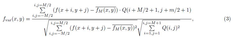
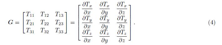
The magnetic anomaly gradient tensor is defined as
Essentially, the proposed kernel function shows the same contribution as the previous one. Both of them are calculated through moving windows, suppress high frequency signal, and in the meantime detect the edge. The differences between them are as follows:
(1)The previous study(Zhang et al., 2011)aims at the magnetic anomalies with vertical magnetization direction, and detects the edge through full scanning.
(2)The improved algorithm aims at the oblique magnetization direction, and detects the edge through the adaptive direction instead of the full scanning.
(3)The ANV method for the RTP field in the previous study uses the second derivative of magnetic field to detect the boundary, while the improved algorithm uses the third derivative of the magnetic field to detect the boundary.
Calculating the improved Anisotropy Normalized Variance(ANV)requires determining the following parameters: the kernel function st and ard deviation σ, the window M, the anisotropy scale cof, and the direction θ.
(1)The kernel function could be understood as a filter function, the st and ard deviation σ has no unit; the size of window M represents the number of points in the window, and also has no unit. In this study, we set σ = M/3.
(2)The size of window is determined by the noise level, a large window can suppress noise, meanwhile it may ignore the information which is less than this window.
(3)For the anisotropy scale, the larger the cof, the larger the difference of the longer and the shorter axis. In the application, when the anisotropy of the source is significant, a large cof will be more conducive to edge detection(usually we set cof=2).
(4)For the direction θ, the adaptive direction calculation will be used in this paper,
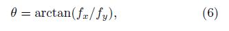
where fx and fy denote the derivatives along x-, and y-direction, respectively.
The algorithm is shown in Fig. 2. If the observed magnetic gradient tensor exists, it can be calculated directly; otherwise we need to compute each component firstly from the observed field △T. The characteristics of this proposed method are as follows:

|
Fig.2 The flowchart of the proposed method |
(1)First, the role of the anisotropic scale cof is equivalent to calculate the horizontal derivative in a local window; it can adaptively determine the ‘derivative direction’ according to the anomalies.
(2)The anisotropic Gaussian function can obtain the potential field derivative, it is also used as a Gaussian smoother to ensure the calculation stability of ‘high-pass filter’.
(3)Based on the gradient tensor module, the improved algorithm can reduce the dependence on the magnetization direction; it can h and le non-vertical magnetization anomalies with unknown magnetization direction. Besides, as mentioned above, this method is equivalent to the third derivative of the magnetic field, and thus, it uses the maximum amplitude to detect the field source boundary.
3 MODEL TESTSWe build a weak magnetic anomaly detection model to verify the proposed method: the offshore marine exploration weak anomaly(Santos et al., 2012). The magnetic anomalies obtained from the forward modeling are shown in Fig. 3a, Fig. 3b is the cross section of the model. Because of the oblique magnetization, the relationship between the magnetic anomalies and the sources is not clear, especially in the weak anomaly area.

|
(a) The modeled magnetic field with an inclination of 15° and a declination of 20°; (b) The section along the profile AA0 shown as the white line in Fig. 3a. Fig.3 The model test with the model locations shown as the black lines |
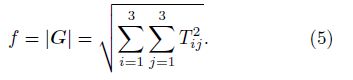
Most previous edge detection methods require vertical magnetization magnetic anomalies, e.g. the Tilt gradient, although it had been applied on the oblique magnetization magnetic anomaly(Santos et al., 2012). As a comparison, we also calculated the Tilt gradient of Fig. 3a, as shown in Fig. 4a. Obviously, this result does not objectively reflect the edge information of the abnormal body. Fig. 4b is the horizontal derivative of the Tilt gradient. Verduzco et al.(2004)indicates that the method is independent of magnetization direction. It shows that the horizontal derivative of Tilt gradient enhances the effect of edge detection, meanwhile it also generates a number of false anomalies. Fig. 5 is the results of the tensor, where values of tensor invariant I1 and tensor Mu are calculated as follows

|
Fig.4 (a) Tilt gradients; (b) Horizontal derivatives of Tilt gradients |

|
(a) 3D analytical signal amplitude; (b) Tensor modules; (c) Invariable of tensor I1; (d) Mu value of tensor. Fig.5 Results of gradients and tensors |
Please refer to Beiki et al.(2012)for the detailed calculation of L1 and L2.
We can found that the tensor results can reduce the effect of oblique magnetization to some extent, and enhance the corresponding relationship between anomalies and field sources. On the other h and , these methods have the properties of high-pass filtering, so they lack the capability for detecting the deep weak anomaly. As shown in Fig. 5, the four results are reflecting the south boundary of the model, but not for the north boundary of the model, also does not reflect the simulated local weak anomaly model(Model 2)clearly.
Figure 6a is the result from the proposed method. The ANV based on tensor mode can not only reduce the effects of oblique magnetization, but also enhance the edge detection of deep weak anomaly. As a comparison, we calculated the ANV based on the 3D analytic signal amplitude(Fig. 6b). Obviously, Fig. 6a is better than Fig. 6b, it indicates that magnetic anomaly tensor model reduces the dependency on magnetization direction better than the 3D analytic signal amplitude in this 3D case.

|
Fig.6 The anisotropy normalized variance based on tensor mode (a), and 3D analytic signal amplitude (b) |
Figure 7a shows a total magnetic field of magnetite exploration from western China. The previous geological and drilling works have verified that this area is an ore-concentrated area. Magnetic properties of rocks and minerals in the area are relatively simple: the iron ore body has strong magnetization, on the other h and the wall rock has no or weak magnetization. The magnetic anomaly on the south side is positive; while the north side has a negative anomaly. We can see that most of the drillholes with known magnetite are located at the gradient magnetic anomaly belt, but the details are not clear. In addition, in the east side of the study area, the drillhole P17-2 has a thick layer of magnetite, while the intensity of magnetic anomaly is just about 200 nT. To find out the location of iron ore body boundaries and provide the basis for the next mining, this research needs to implement fine processing on the magnetic anomaly. In order to avoid the effects of remanence and other uncertainties in ore-concentrated area, this paper directly h and le the observed magnetic anomalies(not the RTP field).

|
Fig.7 (a) Measured magnetic anomalies (not reduction to the pole); (b) Horizontal derivatives of Tilt gradients |
First, Fig. 7b shows the result from the horizontal derivative of Tilt gradient. Similar to Fig. 4b, this method generates some false anomalies, which make it difficult to detect the source edge. Fig. 8 shows the results from the magnetic tensor. All of them reduce the effect of oblique magnetization to some extent. Unfortunately, they are lacking in weak anomaly detection from superimposed anomalies in east side of the study area. Zhang et al.(2013)stated that the main anomalies in this area(located between Line P4-Line P9)are composed of south and north anomalies superposition. There are a number of local magnetic iron ore bodies from Line P9 east to Line P18. These significant features are not shown in the results of Fig. 8.

|
(a) 3D analytic signal amplitude; (b) Tensor module; (c) Invariable of tensor I1; (d) Mu values of tensor. Fig.8 Results of gradients and tensors |
Figure 9a shows the ANV based on tensor module, and Fig. 9b is the ANV based on 3D analytic signal amplitude. By contrast, Fig. 9a reflects the anomaly B better than Fig. 9b. Both of them not only reduce the influence of oblique magnetization and clearly distinguish the two secondary anomalies A and B which are superimposed on the main anomalies, but also improve the weak anomaly detection in east side of the study area. According to Fig. 9a and drillholes’ information, detailed analyses are as follows:

|
Fig.9 The anisotropy normalized variance based on tensor module (a) and 3D analytic signal amplitude (b) |
(1)Drillholes verified that the top depth of iron ore body is between 210~250 m, the thickness of the main iron body is about 30 m, and the ore bodies are veinlike and plate-shaped, NW trending and south-dipping.
(2)For the drillholes with magnetite, the iron body depths in drillholes No.2, No.4 and No.5 on Line P7 are shallower than 300 m, while in drillhole No.1 the depth is about 350 m. Meanwhile, the iron body depth in the drillhole No.3 on Line P8 is 220 m, while the depths in drillholes No.1 and No.2 are nearly 400 m, meanwhile the depth in drillhole No.2 is deeper than drillhole No.1, and the iron ore body becomes thinner. Such characteristics fit well with the results in Fig. 9a.
(3)The Line P9 is located in the saddle between anomalies A and C, the corresponding depth of the ore body in drillhole P9-1 is about 440 m, the thickness is about 4 m.
(4)For the anomaly C, we state that the drillholes P10-3, P11-4, and P11-5 have magnetite, but they are located outside the determined source area from the ANV result, why? First, the drillhole P10-3 with magnetite is a result of the north ore body dipping towards south; second, the depth of the iron body in drillhole P11-5 is about 400 m, and the thickness of the iron body is just 1 m, which shows the ore body dipping towards south. Meanwhile, the local anomalies nearby Line P17 which are difficult to distinguish on the original field are also highlighted, and it is consistent with the drillholes.
5 CONCLUSIONSSince the early 1970s, a lot of researches have been focusing on the edge detection, and many new ideas are proposed. To tackle the complexity of magnetic anomalies, most of the methods are implemented based on the vertical magnetization field or RTP field. While for the magnetic field at low latitude or with unknown magnetization direction, RTP is impossible and thus, these kinds of methods do not work. This paper is focusing on edge detection based on oblique magnetization field, and some insights are obtained as follows:
(1)Most of the traditional edge detection methods are based on the vertical magnetization anomalies, such as the Tilt gradient. If they are applied to oblique magnetization field, it is possible to achieve the ‘Balanced Filter’(highlighting the deep weak anomalies and not suppressing the shallow anomalies at the same time), but it is not able to detect the edge of field source.
(2)For reducing the effect of magnetization direction, the magnetic tensor module works better than the 3D analytic signal amplitude.
(3)Using the anisotropy normalized variance based on the magnetic gradient tensor can detect the source edge from the magnetic field with unknown magnetization direction.
(4)Determination of the top depth based on the edge detection is worthy of further research.
ACKNOWLEDGMENTSThis research was in partial supported by the Sao Paulo State Funding(2012/00593-9), the Fundamental Research Funds for National University, China University of Geosciences(Wuhan)(CUG120815, CUG120501, CUG120116, CUG130103), Chinese Geological Survey Project(12120113101800) and Major State Basic Research Development Program of China(973 Program)(2013CB733200). The authors thank Zhao Yabo and Shuang Liu from China University of Geosciences for the translation.
| [1] | Beiki M. 2010. Analytic signals of gravity gradient tensor and their application to estimate source location. Geophysics, 75(6):159-174. |
| [2] | Beiki M, Pedersen L B. 2010. Eigenvector analysis of gravity gradient tensor to locate geologic bodies. Geophysics, 75(6):I37-I49. |
| [3] | Beiki M, Pedersen L, Nazi H. 2011. Interpretation of aeromagnetic data using eigenvector analysis of pseudogravity gradient tensor. Geophysics, 76(3):L1-L10. |
| [4] | Beiki M, Clark D A, Austin J R, et al. 2012. Estimating source location using normalized magnetic source strength calculated from magnetic gradient tensor data. Geophysics, 77(6):J23-J37. |
| [5] | Clark D A. 2009. Improved methods for interpreting magnetic gradient tensor data. IAGA 11th Scientific Assembly. |
| [6] | Cooper G R J, Cowan D R. 2011. A generalized derivative operator for potential field data. Geophysical Prospecting, 59(1):188-194. |
| [7] | Cooper G R J. 2013. Reply to a discussion about the "Hyperbolic tilt angle method" by Zhou et al. Computers & Geosciences, 52:496-497. |
| [8] | Lahti I, Karinen T. 2010. Tilt derivative multiscale edges of magnetic data. The Leading Edge, 29(1):24-29. |
| [9] | Ma G Q, Huang D N, Yu P, et al. 2012. Application of improved balancing filters to edge identification of potential field data.. Chinese J. Geophys (in Chinese), 55(12):4288-4295. |
| [10] | Nabighian M N. 1972. The analytic signal of two-dimensional magnetic bodies with polygonal cross-section:its properties and use for automated anomaly interpretation. Geophysics, 37(3):507-517. |
| [11] | Oruç B, Sertçelik I, Kafadar Ö, et al. 2013. Structural interpretation of the Erzurum Basin, eastern Turkey, using curvature gravity gradient tensor and gravity inversion of basement relief. Journal of Applied Geophysics, 88:105-113. |
| [12] | Santos D F, Silva J B C, Barbosa V C F, et al. 2012. Deep-pas-An aeromagnetic data filter to enhance deep features in marginal basins. Geophysics, 73(3):J15-J22. |
| [13] | Verduzco B, Fairhead J D, Green C M, et al. 2004. New insights into magnetic derivatives for structural mapping. The Leading Edge, 23(2):116-119. |
| [14] | Wang Y G, Zhang F X, Liu C, et al. 2013. Edge detection in potential fields using optimal auto-ratio of vertical gradient.Chinese J. Geophys. (in Chinese), 56(7):2463-2472. |
| [15] | Zhang H L, Liu T Y, Yang Y S. 2011. Calculation of gravity and magnetic source boundary based on anisotropy normalized variance. Chinese J. Geophys. (in Chinese), 54(7):1921-1927. |
| [16] | Zhang H L, Hu X Y, Liu T Y. 2012. Fast inversion of magnetic source boundary and top depth via second order derivative.Chinese J. Geophys. (in Chinese), 55(11):3839-3847. |
| [17] | Zhang H L, Ravat D, Hu X Y. 2013. An improved and stable downward continuation of potential field data:The truncated Taylor series iterative downward continuation method. Geophysics, 78(5):J75-J86. |
| [18] | Zhou W N, Du X J, Li J Y. 2013. A discussion about hyperbolic tilt angle method. Computers & Geosciences, 52:493-495. |