1 INTRODUCTION

With the fast development of computer science and technology, it is viable for researchers to simulateglobal seismic wave propagation(Komatitsch et al., 2002; Yan et al., 2009; Zhang et al., 2009; Komatitsch et al., 2010; Long et al., 2010). Because of irregular interfaces and rugged free surface of the earth(Komatitsch and Tromp, 2002a, b), traditional finite difference method or pseudo-spectral method with regular grid is notable to correctly fit complex topography(Fornberg, 1987; Moczo et al., 2000; Magnoni et al., 2014). Classicalspectral element method(SEM)chooses GLL(Gauss-Lobatto-Legendre)interpolation points, and constructshigh-order polynomial in the form of Lagrange tensor product, which obtains lumped mass matrix and avoidssolving large scale linear equation system(Wang et al., 2012). Though classical SEM is highly efficient inmodeling seismic wave in global model, quadrilateral elements(hexahedron in 3D case)in SEM are not able toaccurately describe rough interfaces. Though a finer grid can well present boundary variation, computation costmay increase dramatically. SEM with triangular mesh(TSEM)can easily h and le complex geological structures, however it needs more interpolation nodes to obtain acceptable accuracy, as the accuracy of each Koornwinder-Dubiner polynomials is not the same, which leads to a huge global stiffness matrix and hinders the applicationof TSEM in large scale seismic wave simulations. Many optimized methods with satisfactory accuracy havebeen developed based on the traditional methods, such as nearly analytic discretized method(Yang et al, 2003, 2014), convolutional differentiator method(Li et al., 2012) and optimized coefficient finite difference method(Zhang and Yao, 2013), but these methods still suffer from some drawbacks of the traditional methods, such aslow accuracy in modeling surface wave and incapability h and ling rugged topography.

Classical finite element method(FEM)has the power of discretizing a geological model with a mesh ofarbitrary shape elements, however classical FEM with consistent mass matrix(CFEM)is confronted with huge computation costs as the inversion of consistent mass matrix is involved, which decreases the computationefficiency in practical applications. Using mass lumping technique and considering the acceleration in eachelement does not change obviously, we can lump the coupled inertial force to one node, and obtain the lumpedmatrix finite element method(LFEM), which leads to an explicit method. The numerical orders of LFEM and CFEM are the same. LFEM can gain comparable accuracy as CFEM under the condition that element sidelength is much shorter than wave length and numerical integration has sufficient accuracy, or the numericalaccuracy of LFEM may be very low. Marfurt(1984)proposed a new mass matrix(mixed mass matrix)(MFEM)by linearly combining consistent mass with lumped mass, and investigated its accuracy by analyzing its numericaldispersion in solving acoustic wave equation, however MFEM does not lead to an explicit method. In this article, we introduce a residual mass matrix to exp and the inverse of mixed mass matrix into a series based on Taylorexpansion. One can select the first several terms of the series to satisfy different precision requirements.

Few researchers have discussed dispersion properties of FEM with triangular mesh in the literature(Mullen, 1982), and the discussion of dispersion properties is mainly concentrated on square or quadrilateral element grid(Abboud and Pinsky, 1992; Mulder, 1999; Zyserman and Gauzellino, 2005; De Basabe and Sen, 2007, 2010;Zyserman and Santos, 2007; Seriani and Oliveira, 2008). The dispersion properties of TSEM are also paid littleattention for the scheme is hard to construct(Mazzieri and Rapetti, 2012; Liu et al., 2013). It is necessaryto conduct a comprehensive study about dispersion properties of FEM with triangular mesh, and find thedifferences among the above three types of mass matrix in modeling acoustic and elastic wave propagation. Thebehaviors of dispersion are also related to element shape, interpolation order and P- to S-wave speed ratio, and a quantitative discussion is useful for grid generation and parameter setting in practical simulations.

The basis functions along two orthogonal directions are decoupled for FEM with quadrilateral mesh, and the mass matrix can be decomposed into the tensor products of one dimensional mass matrix(Wang, 1993;Zhou et al., 1997). By analyzing the periodicity of mesh, the dispersion relations in 2D case can be expressedin the form of the combinations of dispersion relations in 1D case(De Basabe and Sen, 2007, 2010). The basisfunctions are coupled as area coordinates should satisfy a certain equality, so dispersion relations can not beobtained from 1D relations. Here we construct the generalized eigenvalue problem for FEM with triangularmesh, and analyzing the periodicity of the nodes in a regular mesh, and then infinite order eigenvalue problemcan be simplified to a finite order problem. We discuss the influence factors of dispersion properties, and presentthe dissipation of MFEM at the end of the paper.

2 DISCRETIZING ACOUSTIC AND ELASTIC EQUATIONS BY FEM 2.1 Classical Finite Element Method

The media of the earth is extremely complex. For theoretical analysis and practical application, seismicwave propagation through the earth is usually described by acoustic or elastic equations(Ma et al., 2010, 2011).The acoustic wave equation in heterogeneous medium can be written as

where ▽ =(а/а_x, а/а_z)^T in 2D case, p is pressure field, ρ is density, λ is Lame constant, f is the exterior force, and two dots above p represent second-order temporal derivative. The elastic wave equation in heterogeneousmedium can be expressed as

where u =(u_x, u_z)^T is displacement vector, f is exterior force vector, and μ is another Lame constant.

We need make some assumptions before dispersion analysis. First, exterior force is free; second, themedium is isotropic. Under these assumptions, Eq.(1)can be reduced to

where α = is acoustic wave velocity. Eq.(2)can be simplified as

where α = is the velocity of P-wave, and β = is the velocity of S-wave.

Discretizing Eq.(3)by FEM, multiplying Eq.(3)by an arbitrary test function v, and integrating in thefinite element domain, the following weak form of acoustic equation can be obtained by integration by parts and Green formula.

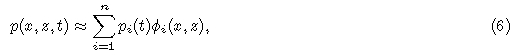
We discretize the spatial domain into N nonoverlappping triangular elements, choose n interpolationnodes in each element, and construct basis function Φ_i(i = 1, 2, · · ·, n). Then the value of pressure field can beapproximately expressed as

where p_i is the value of pressure in the interpolation nodes. The discretized form of Eq.(5)can be written as

where the same subscripts denote summation. M and K are consistent and stiffness matrix, respectively. M and K can be written as

Various temporal schemes can be adopted to solve Eq.(7), such as Lax-Wendroff method with arbitraryeven order(Dablain, 1986; Chen, 2009; De Basabe and Sen, 2010), Runge-Kutta scheme(Chen et al., 2010), Newmark method(Komatitsch and Tromp, 2002a, b) and symplectic methods(Ma et al., 2011; Li et al., 2012;Wang et al., 2012; Liu et al., 2013a, b). Among these methods, central difference(i. e. second-order Lax-Wendroff method)is the most efficient scheme. In the paper, we mainly discuss the spatial discretization, so wesimply choose central difference to discretize Eq.(7), and the fully discretized form of Eq.(7)can be written as

where superscript l denotes temporal level and △t is temporal increment.

Multiplying elastic wave Eq.(4)by a test vector function, integrating over the finite element domain, and using integration by parts and Green formula, we obtain the following weak form equation

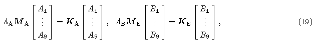
where u =(u_x, u_z)^T, two dots production can be expressed as A : B = A_ijB_ij, and A and B are both m-th order tensors. Eq.(10)can be discretized as

where M, K¹, K², K³ and K⁴ can be written as

where r = V_P/V_S is P to S velocity ratio, Φ_{i, x} = аΦ_i/а_x, and Φ_{i, z} = аΦ_i/а_z.

2.2 Mixed Mass Matrix

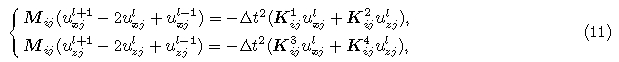
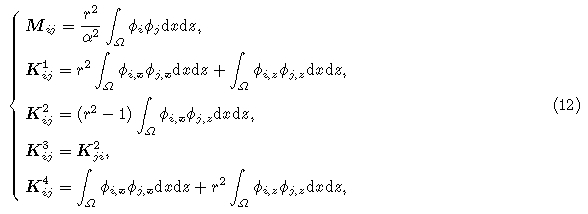
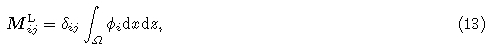
From Eqs.(9) and (11), we can find that classical FEM for modeling seismic wave propagation involvessolving a large linear equation system. In order to reduce computation costs, we often lump the mass matrixto form a diagonal mass matrix based on the assumption that acceleration does not change obviously in eachelement. From the basic theory of FEM, one can easily prove that the error order of this approximation isthe same as that of consistent mass matrix, so convergence rate of lumped mass matrix is nearly the same asthe consistent mass matrix(Fried and Malkus, 1975). But the accuracy of LFEM is inferior to that of CFEM(Mullen and Belytschko, 1982). Lumped mass matrix can be expressed as

where δ is delta function and it is equal to 1 or 0 when subscripts are the same or different, respectively. Toimprove the accuracy of LFEM and maintain its efficiency, according to the method proposed by Marfurt(1984), Seriani and Olivira(2007), we can linearly combine the lumped mass with consistent mass to obtain mixed massmatrix, which can be written as

where a ∈(0, 1). In practical applications, we hope Eq.(14)does not involve solving large linear equationssystem. Here we employ Taylor expansion to exp and the inversion of M^M into series, and use the first several terms to approximate the inverse of M^M. The Taylor series can be written as

where M^F =M -M^L is residual mass matrix. It is easy to prove that the eigenvalues of(M^L)^-1M^F are inthe interval(–1, 0), so the Taylors series converges. Practical computation indicates that the first three termsof Eq.(15)can get preferable results when a = 0.5. In the rest of the paper, we let a = 0.5.

3 DISPERSION ANALYSIS OF ELASTIC AND ACOUSTIC WAVE PROPAGATION

The dispersion property of acoustic and elastic propagation is related to analyzing the generalized eigenvalueproblem, which can be written as Eq.(17). In this section, we discuss the different factors that influencedispersion of FEM with triangular mesh. We can obtain the close form of dispersion relation when first-orderinterpolation is used. However, we can only obtain numerical results when high-order interpolation is employed.Let us consider the plane wave solution of a wave equation:

where A_j is a constant on the j-th node, k is wavenumber, and x_j is the coordinate of the j-th node.

Inserting Eq.(16)into Eq.(9), we obtain the following generalized eigenvalue problem

where

3.1 Dispersion Characteristics of Three Mass Matrix Types

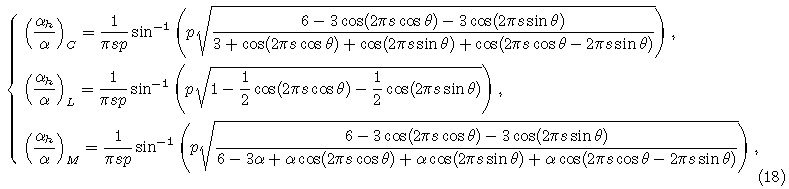
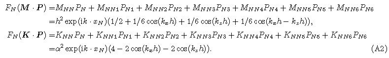
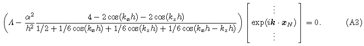
We use isosceles right triangular elements with both side being h to discretize finite element domain, whichis shown in Fig. 1, and we discuss the grid dispersion of the three types of mass matrix in Eqs.(8), (13) and (14).For first order interpolation, the dispersion relations on every node in figure 1 are the same, so the dispersionrelation of any node can represent the global dispersion property, which is proved in Appendix A. From Eqs.(16) and (17), the dispersion relation of CFEM, LFEM, and MFEM for acoustic wave modeling can be written as

where s is sample rate(the reciprocal of the number of grid points per wavelength). θ is the propagationdirection to the vertical axis. p = is stability parameter(Courant number).

From Eq.(18), stability limits of CFEM, LFEM, and MFEM are 0.408248, 0.707107, and 0.577350, respectively.CFEM has the smallest stability range, while LFEM possessesthe largest stability range, and MFEM has a moderatestability range. Fig. 2 shows that three types of massmatrix FEM exhibit the largest numerical dispersion alongcoordinate axis, and smallest dispersion in the directionθ = 45°. In all directions, the numerical velocity of CFEMis larger than physics velocity, while the numerical velocitiesof LFEM and MFEM are both smaller than physicsvelocity. For the amplitude of numerical dispersion, LFEMsuffers from the most severe numerical dispersion, and amplitudeof CFEM is slightly smaller than that of LFEM, while the amplitude of MFEM is the smallest. To keep dispersion error less than 1%, it is suggested to use atleast five points per wavelength in practical simulations. In the following comparisons, we use MFEM to discussthe other influence factors.

3.2 The Effects of Element Shape on Numerical Dispersion

In the process of mesh generation, we need to know the different effects of different element shapes onnumerical dispersion so as to avoid distorted grids and get better numerical results. Besides the mesh in Fig. 1(T1), we choose additional three mesh types to discuss the numerical dispersion of MFEM, which is shown inFig. 3. Fig. 3a is the mesh with equilateral triangular elements(T2), while Fig. 3b and c are other two mesheswith isosceles triangular elements with vertex angle being 30°(T3) and 120°(T4), respectively. For linearinterpolation, we present the numerical dispersion of MFEM in the four meshes in Fig. 4.

We also obtain the stability limits for the three meshes, which are 0.645494, 0.203597, and 0.268643, respectively. The stability properties of MFEM in T1 and T2 are much better than that in T3 and T4. FromFig. 4, one can find that the numerical dispersion in T4 is the smallest when wave propagates along z axis.When the direction of propagation slightly deviates from z axis, the dispersion in T4 becomes very large. Whenpropagation angle equals 60°, the amplitude of dispersion exceeds 40%; the amplitude is larger than 70% whenpropagation angle equals 90°. The dispersion in T2 varies very intensively, especially when the sample rate issmall. The dispersion in T1 and T2 does not change intensively as wave propagating in different directions.During the process of mesh generation, the elements should be close to the isosceles right triangle or equilateral triangle and avoid triangles with small or large degrees of internal angle. Because the area of isosceles righttriangle is times as that of equilateral triangle, using right triangular elements to discretize the finiteelement domain generates fewer elements.

3.3 Effects of Interpolation Order on Numerical Dispersion

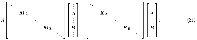
From Sections 3.1–3.2, we can find that MFEM with linear interpolation suffers from large numericaldispersion and anisotropy unless the sample rate is very small. In order to suppress numerical dispersion and anisotropy, high-order interpolations are often employed.In this section, we discuss the numericaldispersion of MFEM with second-order and thirdorderinterpolations in T1 mesh. Fig. 5 depicts theperiodic points for second-order interpolation(solidcircle) and third-order interpolation(empty circle), and one can find the four and nine points periodicallyappear in T1 for second- and third-order interpolations, respectively. Here we select the nine periodicalpoints to discuss the generalized eigenvalue problem.One group of 9 points(denoted as A)can be movedto another group(denoted as B)by a times translationalong x axis and b times translation along z axis. The generalized eigenvalue problem for A and B can be written as

where M_A, M_B, K_A, K_B are mass and stiffness matrices for A and B. The values of these matrices are independentof position, and are only dependent on element shape. Because the element shape is identical in themesh(see Fig. 1), we have M_A = M_B, K_A = K_B, A = [A₁, · · ·, A₉]^T and B = [B₁, · · ·, B₉]^T are the planewave solutions for A and B. Based on the periodicity of the grid, we have the following expression

From Eqs.(19) and (20), we have Λ_A = Λ_B. All the nodes in the grid should satisfy the following generalizedeigenvalue problem

Obviously we have Λ = Λ_A = Λ_B, or the conclusion from Eq.(21)contradicts with Λ_A = Λ_B. The infiniteorder eigenvalue problem can be reduced to ninth order problem. To obtain the close form dispersion relationfor second- or third-order interpolation is extremely hard, but we can get the numerical solution by means ofmathematical software. The results are shown in Fig. 6.

Second- and third-order interpolation can successfully reduce numerical dispersion compared to linearinterpolation. When the sample rate is smaller than 1/3, the dispersion errors are less than 1% and 0.6% forsecond- and third-order interpolations, respectively. The numerical anisotropy of second-order interpolationis much less than that of linear interpolation. The numerical anisotropy of third-order interpolation can beneglected. The dispersion error is mainly controlled by sample rate, and the variation of dispersion errorin different directions is not obvious. From the discussion of this section, it is suggested to use third-orderinterpolation to reduce numerical dispersion.

3.4 The Effects of Wave Speed Ratio on Numerical Dispersion

In Sections 3.1–3.3, we discussed the dispersion of acoustic wave propagation, and the above influencefactors on P- and S-wave in elastic media are nearly the same as acoustic wave, so we does not make a repeated discussion. In this section, we discuss another factor affecting P- and S-wave dispersions in elastic media, whichis wave speed ratio(r)or Poisson ratio. Fig. 7 presents dispersion properties of P- and S-wave when the stabilityparameter p = 0.2 and interpolation is third-order. The directions of P- and S-wave propagation are both alongz axis.

From Fig. 7, we can see that the dispersion amplitude of both P- and S-wave increases as r increases. Theinfluence from r is very small, and the difference of dispersion amplitude between r = 1.7 and r = 8.0 is lessthan 0.5%. The dispersion error of S-wave is slightly larger than that of P-wave. We can also observe that theamplitudes of dispersion error are less than 3.6% and 2.8% for S- and P-wave, respectively, even if s reaches 0.5.

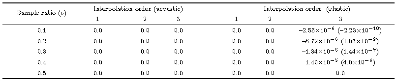
3.5 Numerical Dissipation of MFEM

In Eq.(16), if the characteristic frequency is a complex number by solving Eq.(17), the characteristicfrequency can be written as w_h+iε, in which w_h is numerical frequency. Substituting the characteristic frequencyinto Eq.(16), the imaginary part iε generates numerical dissipation, and the amplitude of plane wave at thenext time instance is e^-ε△t times as that at current time instance. In this section, we present the dissipation ofMFEM using various sample ratios with stability parameter being 0.2 as wave propagating along z axis. Table 1 shows the numerical dissipation of MFEM modeling acoustic and elastic wave(r = 1.7)for different sampleratios and interpolation orders. From Table 1, one can see that MFEM does not show dissipation in acousticcase. For first- and second-order interpolation, MFEM still keeps nondissipative property, while for third-orderinterpolation, both P- and S-wave exhibit dissipation, and generally the dissipation increases as s increases.The dissipation of P-wave is larger than that of S-wave by one order of magnitude, however the " values areextremely small, which is nearly negligible. Here we can come to the conclusion that numerical errors are mainlyfrom numerical dispersion.

4 NUMERICAL EXPERIMENTS

In this section, we conduct three numerical experiments to demonstrate the validity of the analysis above.The size of the first model is 2000 m×2000 m, and the velocity of acoustic wave is 2000 m·s^-1. A source islocated at the center of the model, which is a Ricker wavelet with peak spectrum at 20 Hz. To minimize thedispersion from temporal discretization, we choose a relatively small temporal increment, which is 0.2 ms. Themodel is discretized by T1 mesh, the right angle side length is 10 m. Figs. 8(a–c)show the snapshots of wavefieldat 0.4 s, which are computed by CFEM, LFEM, and MFEM, respectively. In the direction 45° to z axis, strongnumerical dispersions occur in Fig. 8a, and numerical velocity is larger than the physical velocity. In the interiorof wave-front circle, very strong numerical dispersions appear in Fig. 8b. In the direction as that in Fig. 8a, thenumerical dispersions are very weak compared to those in Figs. 8a and b. From this experiment, we verify thatMFEM has great ability in suppressing numerical dispersion.

The parameters of the second experiment are the same as the first experiment except the peak frequencyof Ricker being 35 Hz. We use T2, T3, and T4 meshes to discretize the second model. The snapshots at 0.3 sgenerated by MFEM in T2, T3, and T4 meshes are shown in Fig. 9. One can see that no obvious numericaldispersion occurs in Fig. 9a; in the vertical direction, some weak dispersions exist interior of the wave-frontcircle in Fig. 9b; extremely strong numerical dispersion appears along x axis in Fig. 9c. From the comparison, we conclude that when we generate a finite element mesh, the element shape should be close to regular shape and avoids the deformity shape.

In the third experiment, we examine the dispersion behavior of MFEM modeling P-SV wave in elasticmedia with relatively large wave speed ratio. The size of the third model is 1500 m×1500 m. The velocityof P-wave is 3000 m·s^-1, and the velocity of S-wave is 1000 m·s^-1. The source is vertical force, which is aRicker wavelet with peak spectrum at 20 Hz. We choose T1 mesh to discretize this model. The right angle sidelength is 5 m, 10 m, and 15 m for first-, second-, and third-order interpolation, respectively, and the total nodesafter discretization are the same for different interpolations. The temporal interval is 0.2 ms. The snapshotsof elastic wavefield at 0.2 s are shown in Fig. 10. The shortest wavelength of S-wave is about 20 m, and thenumber of points per shortest wavelength is 4. The snapshot in Fig. 10a is generated by MFEM with first-orderinterpolation, and one can see that the shape of the wave-front of S-wave is an ellipse, and severe numericaldispersion exists in front of the wave-front of S-wave. First-order interpolation presents very bad results and the propagation of elastic wave is not well modeled. When the interpolation becomes second-order, very weaknumerical dispersion exists in front of the wave-front of S-wave in Fig. 10b, and the numerical anisotropy is not visible. When the interpolation becomes third-order, the propagation of P- and S-wave is correctly modeled. Inpractical seismic wave simulations, we suggest using third-order interpolation to suppress numerical dispersion.

5 CONCLUSIONS

In this article, we propose MFEM to model acoustic and elastic wave propagation. The dispersion propertyof MFEM is compared with that of CFEM and LFEM, and the analysis shows MFEM has great ability tosuppress numerical dispersion. Three typical influences on numerical dispersion are discussed when MFEMsimulates wave propagation. We suggest that element shape should be as regular as possible and third-orderinterpolation should be used for spatial approximation. We point out that numerical errors are mainly fromnumerical dispersion and numerical dissipation is negligible.

We adopt simple meshes with regular element for discussion. In practical seismic wave modeling, the meshmay be composed of very complex elements, and the discussion about numerical dispersion in this kind of meshmay be impossible. But we can use the conclusions of this paper to speculate the tendency of the numericaldispersion in a complex mesh.

Special thanks are given to Professor Zhang Huai for his constructive comments of the original manuscript.Valuable suggestions from the two anonymous reviewers are also acknowledged. We are grateful to editor HuSufang for her careful reading and finding the mistakes of the paper. This work was supported by the NationalNatural Science Foundation of China(41174047 and 40874024).

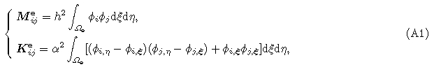
If we use a linear interpolation in Eq.(9) and transform the integration from physics element to referenceelement, the element consistent mass matrix and stiffness matrix can be written as

where η and ξ are local coordinates in reference element. We denote any node in T1 mesh as N, and denote thefirst node in the right h and side as N₁. The rest five anticlockwise nodes around N are denoted as N₂, N₂, N₂, N₅ and N₆, respectively. Function F_N(A) denotes selecting the nth element of vector A. From Eq.(A1), we have

Substituting Eq.(A2)into(17), we have the following equation

The sufficient and necessary condition for(A3)is the following equation

From(A1), we can conclude that the solution to generalized eigenvalue problem of Eq.(17)is unique. Usingthe expression of Λ in Eqs.(17) and (A4), we can obtain the first equation in Eq.(18). The rest two equationsin Eq.(18)can be deduced in the same way.