 2014, Vol. 57


2. Key Laboratory of Cloud-Precipitation Physics and Sever Storms, Institute of Atmospheric Physics, Chinese Academy of Sciences, Beijing 100029, China;
3. National Centers for Environmental Prediction, National Oceanic and Atmospheric Administration, Maryland 20746, USA
Deep convective system which has strong updrafts can transport heat, moisture and hydrometeor verticallyfrom low to high level, and can cause heavy rainfall locally, release latent heat, and produce instantaneous gale.Besides, anvil cirrus forms at the top of updrafts of deep convective system and can exist long time after theconvective system weakening, thus influencing global climate change through adjusting atmospheric radiationbalance.
Houze(1993)showed that updrafts in deep convective systems lift the hydrometeor from low level to upperlevel of convective system, where anvil cirrus forms because of hydrometeor aggregation. Many researchers alsostudied the relationship between formation of anvil cirrus and the deep convective system. For example, Massieet al.(2002)found that about one half of tropical anvil cirrus are caused by the advectional current at the top ofconvective systems. Luo and Rossow(2004)come to the conclusions that entrainment markedly influences theformation of anvil cirrus and the anvil cirrus can be transported to the area 600~1000 km away from convectivesystems. Rickenbach et al.(2008)studied a case of convection and concluded that anvil cirrus forms at thetop of convective system, develops at downstream of convection, and matures about 1~2 hours after convectivesystem dissipated, while the area gets to the maximum.
The TropicalWarm Pool International Cloud Experiment(TWP-ICE)is aimed to studying the microphysicalcharacteristics of convective hydrometeor and their impacts on global climate change. TWP-ICE obtainedabundant observational data through regular and irregular observation instruments like radar, sounding and aircrafts, which lay a foundation for improvement of Numerical Weather Prediction(NWP)models and convectiveparameterization scheme in numerical models(May et al., 2008). From then on, lots of scientists carried outresearch with the TWP-ICE database. Jin et al.(2007) and Li et al.(2009)used the TWP-ICE data to simulatethe weather system and conducted sensitive experiments with numerical models. Davies et al.(2013)usedan ensemble of large-scale data of TWP-ICE to perform best estimate ensemble single-column models(SCMs)simulation, and found that ensemble simulation enables more complete model investigation compared to traditionalSCM simulation. Wang et al.(2009)tested a new 2-moment microphysics parameterization schemein Community Atmosphere Model(CAM)with TWP-ICE large-scale data, and showed that cloud propertiesin 2-moment scheme can respond reasonably to the changes in the concentration of aerosols and place moreemphasis on the importance of correctly simulating aerosol effects in climate models for aerosol-cloud interactions.Frederick and Schumacher(2008)studied the characteristics of tropical anvil areal coverage, height, and thickness during TWP-ICE with C-b and radar data, and analyzed the morphology, evolution, longevity of theanvil, and the relationship of the anvil with the rest of the precipitating system. Wu et al.(2009)made simulationwith the Weather Research and Forecasting Model(WRF) and Goddard Institute for Space Studies SingleColumn Model(GISS SCM), and found that entrainment strength and updraft strength vary with microphysicsschemes and hydrometeor profiles are sensitive to assumptions of the ice phase microphysics. Studies of Li etal.(2012) and Lin et al.(2012)showed that convective parameterization schemes are the key to simulate cloudwell in climate model. Wang and Liu(2009) and Mrowiec et al.(2012)all analyzed updraft of convection forCloud-Resolving Model(CRM)simulations in their studies. Wang and Liu(2009)pointed out that updraftformations from CRM simulation are so different from those in CAM’s deep convective parameterizations, whichassume that mass flux for a single updraft increases exponentially with height to its top and detrainment isconfined only to a thin layer at the updraft top. As a result, CAM’s assumptions may cause excess moisture and heat transported to the upper troposphere.
Lagrangian methods are usually applied in the study of pollutant dispersion. Furthermore, many researchersemployed these methods to study transportation from troposphere to stratosphere(Chen et al., 2010;Chen et al., 2012) and mesoscale dry intrusion(Gao et al., 2010). Compared with traditional Euler methods, Lagrangian methods can characterize the variation of air motion obviously by ascertaining source and sinkregion. However, few studies among those mentioned above analyzed the transportation characteristics of singleconvective system with Lagrangian methods, and how hydrometeor transportations of deep convective system impact anvil formation. Many studies(e.g., Li et al., 2012; Lin et al., 2012; Wang and Liu, 2009)also haveproved that defects of parameterizations limited the development of numerical models. This paper focuses onthe defects of convective parameterization and studies the characteristics of Lagrangian transportation in atropical deep convective process during TWP-ICE with Lagrangian methods. The results from this paper willlay a preliminary foundation for improvement of model parameterization schemes.
2 DATA AND METHODNon-hydrostatic mesoscale model WRFV3.4.1 is used in this paper to simulate the weather systems duringTWP-ICE from 19 January to 31 January, 2006. Large-scale forcing data employed in WRFV3.4.1 model isNCEP FNL(Final)Operational Global Analysis data on 1-degree by 1-degree grids. Four nested domainsare used. The grid spacing of each domain from outmost to innermost is 30 km, 6 km, 2 km and 0.667 km, respectively. Centers for all four domains are set at Darwin site, Australia(12.425°S, 130.891°E). The area ofinnermost domain encompassing whole TWP-ICE field is about 316 km×316 km. The top of the domain is at10 hPa. Seventy-two vertical levels are employed with vertical grid spacing varying from 70 m near the surfaceto 1000 m near the top of domain. Because the innermost domain can resolve the convective system in cloudresolvingscale, “WRF-CRM” will be used to refer to the innermost domain simulation hereafter. Fig. 1 showssimulation domain. In the figure, shading represents terrain height, six dots represent TWP-ICE observationsites, and pentagon represents TWP-ICE observation domain.

|
Fig. 1 Schematic diagram of simulation domain Shading represents terrain height, pentagon represents TWP-ICE domain and dots represent observation sites. |
The microphysics option chosen in this paper is WSM6 scheme. RRTM and Dudhia schemes are chosenas long wave and short wave radiation options respectively. Choices of boundary layer and l and -surface optionsare YSU scheme and unified Noah scheme respectively. Setup of sub-grid parameterization schemes is similar tothat of Wang and Liu(2009)except for microphysics options. Wang and Liu(2009)chose Thompson scheme, while this paper chose WSM6 scheme. The reason why we choose WSM6 scheme is that Thompson schemesubstantially overestimates the snow content and hence produces biases in cirrus clouds simulations and WSM6scheme has a better representation of cirrus clouds than Thompson scheme(Wang et al., 2009).When studying the characteristics of convective transportation, FLEXPART dispersion model is employedto analyze the WRF-CRM results outputting every five minutes. FLEXPART dispersion model simulatesatmospheric air motion through ascertaining air motion trajectories(Stohl et al., 2005). FLEXPART dispersionmodel generally adopts the simple “zero acceleration” scheme, X(t + △t)= X(t)+ v(X, t)· △t, which canbe used in simulation of long-range and mesoscale transport, diffusion, dry and wet deposition from differentatmospheric release sources. In FLEXPART model, forward modeling calculates the trajectories of air particlesmotion, while backward modeling calculates the source-receptor relationship. Compared with other Lagrangianmodel, FLEXPART dispersion model even takes mesoscale convection and turbulence process into account(Forster and Stohl, 2007). Domain-filling option in FLEXPART dispersion model is also selected to simulate airmotion with WRF-CRM results. Domain-filling means that according to air density, air in a limited 3D area isdivided into a certain number of air particles and each particle has the same mass. In this paper, air in WRFCRMdomain is divided into 600000 air particles. These air particles are driven to move with atmospheric fieldlike temperature, air pressure, wind and humidity from WRF-CRM. Trajectory is calculated by ascertainingpositions of different particles at different moments.
3 SIMULATION RESULTS 3.1 Simulation VerificationFigure 2 shows the comparisons of cloud fraction at different heights from WRF simulation, observations and multi-CRM simulation mean results. Cloud in TWP-ICE is observed by using cloud radar and other remotesensors and cloud fraction is estimated by using ARSCL algorithm(Clothiaux et al., 2000)with radar or otherremote sensors observations. Wang and Liu(2009)pointed out that cloud radars tend to miss high-altitudeclouds and underestimate the cloud top height due to radar signals decaying with distance. Given this fact, cloud fraction simulated by WRF(Fig. 2a)is consistent with observation(Fig. 2b)except for the large differenceon 24 and 25 July, 2006 which were caused by the inconsistency between large-scale forcing field and observation(Wang and Liu, 2009). Cloud fraction from multi-CRM mean results(Fig. 2c)is similar to that from WRFsimulation, especially, the multi-CRM mean fraction is also inconsistent with observation but consistent withWRF simulation of 24 and 25 July, 2006. As a conclusion, WRF model simulates the cloud characteristicsduring TWP-ICE well and the results from WRF simulation can be used in subsequent studies and analyses.

|
Fig. 2 Cloud fraction comparisons among (a) WRF simulation, (b) observation and (c) multi-CRM mean Rectangle in (a) represents WRF-CRM period. |
The main objective of TWP-ICE is to observe and study convective cloud and anvil cirrus related withconvective system. During the observing period, a large amplitude Madden-Julian Oscillation(MJO)eventmoved through the experiment region. Four distinct convective regimes were sampled. These regimes beganwith convectively active monsoon conditions, followed by a suppressed monsoon, three days of clear skies, and then a break period(May et al., 2008). By late 23 January the monsoon trough was receding to the north ofDarwin site, and a large Mesoscale Convective System(MCS)developed in the experiment region and produceddistinct rotation as it moved toward the sea west of Darwin. Fig. 3 shows the simulated meteorology conditionsfor sea surface level and 500 hPa at 21 o’clock 23 and 24 January, 2006. The weather feature reproduced byWRF model is same with those from TWP-ICE experimental weather records and literatures reported(May et al., 2008). Analyzing the sea level pressure and geopotential height fields at 500 hPa, the low-pressure system was located at the sea northeast of Darwin on the 23rd, as the system moved southward, the system was atthe area nearby Darwin site on the 24th. Influenced by the low-pressure system, warm and wet westerly windswere experienced at Darwin site, which caused Darwin site and even whole experiment region becoming wetter.Such high humidity weather state provided favorable conditions for precipitation causing convective systems todevelop. From 23 to 25 January, 2006, as the convective system developing actively, subsequent studies willfocus on the convective systems during this period.

|
Fig. 3 Pressure (potential height) (contours), relative humidity (shaded) and wind field (vector) at sea surface (a, c) and 500 hPa level (b, d) at (a, b) 21 o’clock, 23 January and (c, d) 21 o’clock, 24 January 2006 Black dot represents Darwin station. |
Updraft property of convective system determines how mass, hydrometeor and energy are redistributedduring convective process. Stronger updraft can bring more hydrometeor to upper troposphere. Mass flux meansthe content value of hydrometeor lifted by updraft through a unit area and it is calculated as Mi = ρi ·wi, wherethe subscript i represents the i-th updraft, ρi represents density of updraft and wi represents vertical velocityof updraft. Greater value of mass flux means more hydrometeor be transported by updraft. Vertical variationof mass flux 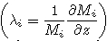 can be used to express entrainment rate of updraft which means the quantity ofmass exchange between updraft and environment. λi > 0 means hydrometeor entrained to convective system and λi < 0 means hydrometeor detrained to environment. Different convective updraft can reach differentheights, and to study the properties of updrafts with different updraft top heights, the same method is adoptedin this paper as Wang and Liu(2009)used for studying mass flux profile of updrafts with different updraft topheights. Fig. 4a shows updrafts mass flux profile from WRF-CRM. Maximum value of mass flux occurs nearthe top of conditional unstable layer, above which the value of mass flux decreases with height. These resultsare similar to those of Wang and Liu(2009).

|
Fig. 4 Comparison of (a) WRF-CRM simulated and (b) CAM assumed normalized mass flux profile of updrafts with different updraft top heights Gray shading represents the top of the conditional unstable layer, Mui represents mass flux of all height updraft and Mbi represents mass flux at updraft base. |
Convective parameterization schemes based on mass flux(Zhang and McFarlance, 1995)are adopted bymany numerical weather models and climate models(e.g., CAM). Those schemes assume that detrainment is confinedjust in a thin layer at the updraft top and the fractional entrainment rate is constant  .Based on these assumptions, Fig. 4b shows the CAM assumed mass flux profile with different updraft top heights.From this figure, we can find that mass flux increases with height till updraft top and this mass flux propertymight cause more hydrometeor be transported to upper troposphere. Wang and Liu(2009)believed that onlyby stratifying the condition such that vertical velocity increases with height can mass flux increase with height.However, dragged by hydrometeor and influenced by updraft turbulence, vertical velocity cannot increase withheight. By the way, the net buoyancy force, a key factor to keep vertical velocity increasing with height, alwaysdecreases with height above conditional unstable layer and this also cannot sustain increasing vertical velocity.As a result, climate models which adopt mass flux scheme(e.g., CAM)cannot give a realistic mass flux profilejust as WRF-CRM do, and this ideal mass flux profile may lead unrealistic cloud simulation. In order to laya preliminary foundation for convective parameterization schemes, discuss will be done in Section 4 throughanalyzing the characteristics of Lagrangian transportation for a convective system.
With WRF-CRM simulation meteorological fields, this paper employs FLEXPART dispersion model to calculate the Lagrangian trajectories. In order to thoroughly study how hydrometeor in convective system istransported, we select air particles with high initial radar reflectivity from a 10 km×10 km horizontal area invertical range from 1.5 km to 8 km during a representative convective process(20 o’clock 24 January–07 o’clock25 January). Fig. 5 shows the percentage of air particles from different initial heights and the percentage of thosecan reach 13 km height. Analyses from Fig. 5 show that as air density decreases with height, the percentageof air particles also decreases with height. In contrast, the percentage of air particles having ability to reachupper troposphere(~13 km)increases with height, and it increases from 30.23% low level to 80.50%. Sucha percentage distribution implies that air particles from higher level can be more easily transported to uppertroposphere.

|
Fig. 5 Distribution of number percentage of air particles from different initial heights (light color) and contribution percentage of particles those can reach 13 km height (dark color) |
Figure 6 shows the scatter plots of horizontal transport distance vs. vertical transport height. From Fig. 6, it is easily found that the furthest distance and highest height air particles can reach are over 300 km and 18km respectively. Gray shading in Fig. 6 represents the top of conditional unstable layer and black solid linerepresents the distance 50 km away from initial points beyond which the air particles are considered to betransported out of the convective system. Preceding analyses show that in convective parameterization schemesonly at the top of updraft hydrometeors are transported out of the convective system, but Fig. 6 has proved thatduring transportation, air particles are already out of convective system around the top of conditional unstablelayer, and it emphasized again the results given in Fig. 4a that hydrometeor from convective system has alreadybeen transported into environmental atmosphere before reaching the top of updraft.

|
Fig. 6 Scatter plots of horizontal transport distance vs. vertical transport height of air particles from different initial heights at (a) 1.5~2 km, (b) 2~3 km, (c) 3~4 km, (d) 4~5 km, (e) 5~6 km, (f) 6~7 km and (g) 7~8 km Gray shading represents the top of the conditional unstable layer and black solid line represents 50 km horizontally away from the initial location of air particles. |
Another typical trait of Fig. 6 is that air particles are transported in both horizontal and vertical directionsbelow 13 km, but transported only in horizontal direction above 13 km. The research of Frederick and Schumacher(2008)has showed that 13 km could be regarded as the height where anvil cirrus stays. Considering thisconclusion and Fig. 6, we can infer that vertical air flow or convective updraft bring hydrometeor to anvil area, and horizontal air flow brings hydrometeor further where hydrometeor may play a significant role in exchangebetween troposphere and stratosphere.
Figures 7 and 8 show the relationships between transport duration and vertical transport height and between transport duration and horizontal transport distance, respectively. From Fig. 7, we can find that mostair particles are transported to 13 km where anvil cirrus stays in 120 minutes, and after 200 minutes all particlesincluding those transported longer are transported to the highest height they can reach. After getting highest, air particles are transported horizontally as Fig. 6 discussed.

|
Fig. 7 Same as Fig. 6, but for scatter plots of transport duration vs. vertical transport height of air particles Gray shading represents the top of the conditional unstable layer, horizontal solid line represents 13 km heights and vertical solid line represents 120 min. |
Figure 8 shows the relationship between transport duration and horizontal transport distance and theblack solid line in the figure represents the linear regression line between air transport duration and horizontaldistance. The slope of regression line is rc, and greater value of rc represents air particles will be transported tofurther in shorter time. Great differences of features during air particles horizontal transportation from differentinitial heights are found in Fig. 8. Expect for the air particles from initial heights 1.5~2 km, air particles fromhigher initial heights will be transported more quickly, because value of rc increases with initial height.

|
Fig. 8 Same as Fig. 6, but for scatter plots of transport duration vs. horizontal transport distance of air particles Black straight line represents the regression line between transport duration and horizontal transport distance and value of rc represents the slope of regression line. |
Another interesting difference is that as initial height increases the discrete degree of air particles in thefigure decreases gradually. Wind turbulence is the possible contributor to this phenomenon. Wind directions inlower level are less uniform than those in upper level, so air particles from lower initial height more easily moveto all direction with steering current, and as a result, air particles from lower initial height are transported morediscretely. Influenced by turbulent winds, some hydrometeor is transported back into convective system againafter being transported into environmental atmosphere.
Figure 9 is the time series of some meteorological variables(e.g., vertical height, specific humidity, airdensity and temperature)at each Lagrangian point, and the horizontal and vertical dash lines represent criticalvalues of different variables and critical time 120 minutes. The result that hydrometeor be transported to thelevel 13 km height around 120 minutes from Fig. 9a is similar with that from Fig. 6. After 120 minutes, theheight of vertical levels where hydrometeor reached varies little around 13km. When the height of hydrometeorincreases, the amount of liquid hydrometeor decreases. Specific humidity(Fig. 9b)decreases with time quicklyto 0.7 g·kg-1 at 120 minutes and 0 g·kg-1 after 120 minutes. Same as specific humidity, air density(Fig. 9c)alsodecreases with time. When hydrometeor particles reach to 13 km height at 120 minutes, air density decreasesto 0.3 g·kg-3; beyond this time the hydrometeor particles maintain at 13 km height, and the air density is alsostabilized around 0.3 g·kg-1. The variation of air temperature is basically similar with those of specific humidity and air humidity, when hydrometeor particles reach to around 13 km height, air temperature decreases to -54°C. Different with other variables, air temperature is more sensitive to the variation of hydrometeor particleswith height. As the height of hydrometeor particles increase or decrease, air temperature also decreases orincreases and finally stabilizes at -54°C. Summarizing the analyses above, we can give a critical characteristicsof convective hydrometeor transportation, after 2 hours transportation of hydrometeor particles, they can reach13 km height level and the environmental values of specific humidity, air density and air temperature are0.7 g·kg-1, 0.3 g·kg-3 and –54°C respectively.

|
Fig. 9 Time series of (a) vertical height (km), (b) specific humidity (g·kg-1), (c) air density (kg·m-3) and (d) temperature (°C) at air particles Lagrange points Horizontal dash line represents critical values of different variables and vertical dash line represents 120 minutes. |
Section 4.1 only analyzes the characteristic of hydrometeor transportation in convective system. To analyzehow hydrometeor transportation in convective system impacts on surrounding environment and developmentof anvil cirrus, this paper calculates the grid air particles transportation frequency with interpolating eachtrajectory points into 5 km×5 km grids. Grid air particles transportation frequency is defined as the ratioof total amount of air particles to the amount of air particles passing through each grid. Fig. 10 shows thedistribution of air particles transportation frequency from different initial heights, and this distribution canguide us to comprehend questions concerning the trajectory of hydrometeor transportation and the impact areaof convective hydrometeor.

|
Fig. 10 Distribution of air particles transportation frequency from different initial heights at (a) 1.5~2 km, (b) 2~3 km, (c) 3~4 km, (d) 4~5 km, (e) 5~6 km, (f) 6~7 km and (g) 7~8 km Black box represents the position of the convective system. |
Controlled by environmental southwest current, hydrometeor is mainly transported in northeast direction, but there are also a few differences among trajectories from different initial height. Fig. 10a shows the distributionof air particles transportation frequency from initial 1.5~2 km and it can be found that a few hydrometeorconveyed to the convective system upstream direction(southeast direction). As the initial height increases, frequency of transportation of hydrometeor to upstream direction decreases. The reason why hydrometeor istransported to upstream is that wind turbulence in lower level is greater than that in upper level, and the windturbulence causes a few hydrometeor particles being conveyed to the convective system upstream.
Figure 10 shows that the furthest distance hydrometeor in convective system can be transported intoenvironment is about 200~300 km where the convective systems plays a role in moisture exchange between troposphere and stratosphere. Analyses of air particles transportation frequency show that except for the area50 km away from initial position, the area most influenced by the convective system is 50~150 km downstreamfrom the deep convective system where the transportation frequency is greater than 10%. Horizontally, themost influenced area is just the anvil area closely associated with convective system, so it can be estimated thatabout 10%~20% of the hydrometeor has an important influence on the anvil cirrus formations.
However, the data used in this paper is from numerical model which has some uncertainties and themicrophysical characteristics have significant impact on anvil cirrus formation. As a result, we still need afurther study of quantitative estimation of the influence of convective system on anvil cirrus development.
Similar with Fig. 10, Fig. 11 shows the distribution of air particle transportation duration time on 5 km×5km grids and its overall distribution is same with the distribution of air particles transportation frequency.Analyses of Fig. 11 show that the area 100~200 km away from convective system has longer duration timebasically greater than 4 hours and the longest can reach 6 hours. Longer duration time area coincides withthe higher air transportation frequency area which just happens to be the anvil area closely associated withconvection. So we can come to the conclusion that the time scale of convective systems impacting on environment and anvil cirrus formation is about 4~6 hours.

|
Fig. 11 Same as Fig. 10, but for distribution of air particle duration time Black box represents the position of the convective system. |
High resolution mesoscale model WRFV3.4.1 is used to simulate the deep convective process duringTWP-ICE. Simulation data from the forth nested domain outputted every five minutes and the FLEXPARTLagrangian dispersion model are employed to study the characteristics of convective transportation. The conclusionsare as follows:
Firstly, WRF model of high resolution can be used in cloud-resolving scale simulation. The cloud characteristicsfrom simulation results are consistent with those observed during TWP-ICE.Secondly, analyses of the Lagrangian characteristics of hydrometeor and the vertical variation of convectiveupdraft mass flux show that convective hydrometeor has already been detrained near conditional unstablelayer, which is inconsistent with convective parameterizations based on mass flux scheme, but consistent withobserved fact. This difference indicates that current convective parameterization scheme may overestimate thehydrometeor contribution of convective systems to upper troposphere.
Thirdly, after two hours, convective hydrometeor is transported to 13 km height and the environmentalvalues of specific humidity, air density and air temperature are 0.7 g·kg-1, 0.3 g·kg-3 and –54°C respectively. Around 13 km height, hydrometeor is mainly transported in horizontal direction and hydrometeor with higherinitial height can be transported further in shorter time.
Finally, the analysis of hydrometeor transportation trajectories shows that hydrometeor transportation ismainly along the steering current direction and the farthest distance hydrometeor can reach is 200~300 km.About 10%~20% of the hydrometeor has an important influence on the anvil area 50~150 km downstreamfrom the deep convective system, of which the time scale is 4~6 hours. However, influenced by low level winddisturbance, some hydrometeor is also conveyed to upstream.
This paper discusses the relationship between hydrometeor Lagrangian transportation and anvil cirrusformation and also draws some preliminary conclusions which may lay a foundation for improving convectiveparameterization. However, sub-grid parameterizations in current NumericalWeather Prediction(NWP)modelshave some problems which may cause uncertainties in evaluating hydrometeor transportation in convectivesystems. Only by quantitative evaluation can we make improvement in convective parameterization schemes, so we still need further study of hydrometeor transportation of different convective system types based on moreaccurate and extensive observation data.
This work was supported by the National Key Basic Research and Development Project of China(2013CB-430103 and 2011CB403405), the National Natural Science Foundation of China(41075039 and 41375058), thePriority Academic Program Development of Jiangsu Higher Education Institutions(PAPD), and the Programfor Excellent Scientific and Technological Innovation Team of Jiangsu Higher Education(2012).
| [1] | Chen B, Xu X D, Bian J C, et al. 2010. Sources, pathways and timescales for the troposphere to stratosphere transport over Asian Monsoon Regions in Boreal Summer. Chinese Journal of Atmospheric Sciences (in Chinese), 34(3):495-505. |
| [2] | Chen B, Xu X D, Yang S, et al. 2012. On the characteristics of water vapor transport from atmosphere boundary layer to stratosphere over Tibetan Plateau regions in summer. Chinese J. Geophys. (in Chinese), 55(2):406-513. |
| [3] | Clothiaux E E, Ackerman T P, Mzce G G, et al. 2000. Objective determination of cloud heights and radar reflectivities using a combination of active remote sensors at the ARM CART sites. J. Appl. Meteor., 39(5):645-665. |
| [4] | Davies L, Jakob C, Cheung K, et al. 2013. A single-column model ensemble approach applied to the TWP-ICE experiment.J. Geophys. Res., 118(12):6544-6563, doi:10.1002/jgrd.50450. |
| [5] | Forster C, Stohl A. 2007. Parameterization of convective transport in a Lagrangian particle dispersion model and its evaluation. J. Appl. Meteor. Climatol., 46(4):403-422. |
| [6] | Frederick K, Schumacher C. 2008. Anvil Characteristics as Seen by C-POL during the Tropical Warm Pool International Cloud Experiment (TWP-ICE). Mon. Wea. Rev., 136(1):206-222. |
| [7] | Fridlind A M, Ackerman A S, Chaboureau J P, et al. 2012. A comparison of TWP-ICE observational data with cloudresolving model results. J. Geophys. Res., 117(D5):D05204, doi:10.1029/2011JD016595. |
| [8] | Gao S T, Yang S, Chen B. 2010. Diagnostic analyses of dry intrusion and nonuniformly saturated instability during a rainfall event. J. Geophys. Res., 115(D2):D02102, doi:10.1029/2009JD012467. |
| [9] | Houze R A. 1993. Cloud Dynamics. New York:Academic Press, 573. |
| [10] | Jin L J, Yin Y, Wang P X, et al. 2007. Numerical modeling of tropical deep convective anvil and sensitivity test on its response to changes in the cloud condensation nuclei concentration. Chinese Journal of Atmospheric Sciences (in Chinese), 31(5):793-804. |
| [11] | Li J P, Yin Y, Jin L J, et al. 2009. A numerical study on deep tropical convection using WRF model. Journal of Tropical Meteorology (in Chinese), 25(3):287-294. |
| [12] | Li L J, Xie X, Wang B, et al. 2012. Evaluating the Performances of GAMIL1.0 and GAMIL2.0 during TWP-ICE with CAPT. Atmos. Oceanic Sci. Lett., 5(1):38-42. |
| [13] | Lin Y L, Donner L J, Petch J, et al. 2012. TWP-ICE global atmospheric model intercomparison:Convection responsiveness and resolution impact. J. Geophys. Res., 117(D9):D09111, doi:10.1029/2011JD017018. |
| [14] | Luo Z Z, Rossow W B. 2004. Characterizing tropical cirrus life cycle, evolution, and interaction with upper-tropospheric water vapor using Lagrangian trajectory analysis of satellite observations. J. Climate, 17(23):4541-4563. |
| [15] | Massie S, Gettelman A, Randel W, et al. 2002. Distribution of tropical cirrus in relation to convection. J. Geophys. Res., 107(D21):AAC19-1-AAC19-16, doi:10.1029/2001JD001293. |
| [16] | May P T, Mather J H, Vaughan G, et al. 2008. The tropical warm pool international cloud experiment. Bull. Amer.Meteor. Soc., 89(5):629-645. |
| [17] | Mrowiec A A, Rio C, Fridlind A M, et al. 2012. Analysis of cloud-resolving simulations of a tropical mesoscale convective system observed during TWP-ICE:Vertical fluxes and draft properties in convective and stratiform regions. J. Geophys.Res., 117(D19):D19201, doi:10.1029/2012JD017759. |
| [18] | Rickenbach T, Kucera P, Gentry M, et al. 2008. The relationship between anvil clouds and convective cells:A case study in south Florida during crystal-face. Mon. Wea. Rev., 136(10):3917-3932. |
| [19] | Sheng P X, Mao J T, Li J G, et al. 2003. Atmospheric Physics (in Chinese). Beijing:Peking University Press, 310-352. |
| [20] | Stohl A, Forster C, Frank A, et al. 2005. Technical note:The Lagrangian particle dispersion model FLEXPART version 6.2. Atmos. Chem. Phys., 5(9):2461-2474. |
| [21] | Varble A, Fridlind A M, Zipser E J, et al. 2011. Evaluation of cloud-resolving model intercomparison simulations using TWP-ICE observations:Precipitation and cloud structure. J. Geophys. Res., 116(D12):D12206, doi:10.1029/2010JD015180. |
| [22] | Wang W G, Liu X H, Xie S C, et al. 2009. Testing ice microphysics parameterizations in the NCAR community atmospheric model version 3 using tropical warm pool-international cloud experiment data. J. Geophys. Res., 114(D14):D14107, doi:10.1029/2009J D14107. |
| [23] | Wang W G, Liu X H. 2009. Evaluating deep updraft formulation in NCAR CAM3 with high-resolution WRF simulations during ARM TWP-ICE. Geophys. Res. Lett., 36(4):L04701, doi:10.1029/2008GL036692. |
| [24] | Wang Y, Long C N, Leung L R, et al. 2009. Evaluating regional cloud-permitting simulations of the WRF model for the Tropical Warm Pool International Cloud Experiment (TWP-ICE), Darwin, 2006. J. Geophys. Res., 114(D21):D21203, doi:10.1029/2009JD012729. |
| [25] | Wu J B, Del Genio A D, Yao M S, et al. 2009. WRF and GISS SCM simulations of convective updraft properties during TWP-ICE. J. Geophys. Res., 114(D4):D04206, doi:10.1029/2008JD010851. |
| [26] | Zhang G J, McFarlane N A. 1995. Sensitivity of climate simulations to the parameterization of cumulus convection in the Canadian Climate Center general-circulation model. Atmos.-Ocean, 33(3):407-446. |