 2014, Vol. 57


Radon transform is widely used in a range of applications in seismic data processing, such as multipleattenuation(Wang, 2003; Schonewille and Aaron, 2007; Xiong et al ., 2009), de-noise(Gong et al ., 2009), wavefieldseparation(Zeng et al ., 2007; Feng et al ., 2011), data interpolation and reconstruction(Wang et al ., 2006;Wang et al ., 2007), velocity dispersion analysis(Pan et al ., 2010), migration and imaging(Huang et al ., 2004), etc. According to the characteristics of the research problem, Radon transform based on the integration methodhas several flexible and diverse forms of transform, such as linear Radon transform( τ-p transform), parabolicRadon transform, hyperbolic Radon transform and polynomial Radon transform(Niu and Sun, 2001). Fordifferent physical fields, a suitable transform should be selected to achieve the optimal solution of the problem.
The more the Radon domain signal and noise energy are concentrated, the better the signal and noise areseparated. For homogeneous horizontal layered media, the hyperbolic Radon transform has higher resolutionthan the others. Moreover it was used to demultiple in marine data(Wang, 2003). Because the subsurfacemedia is commonly anisotropic, the energy propagation and distribution of the seismic wavefield are diverse indifferent directions. In vertical transverse isotropic media(VTI), the travel time curve of the reflection eventis non-hyperbolic according to the anisotropic parameters. Additionally, the seismic data with large offset inisotropic media also has a non-hyperbolic travel time curve. In both situations, the hyperbolic Radon transformcannot guarantee that the reflection energy is converging to separate the signal from noise.
In this paper, we present the anisotropic Radon transform consisting of three parameters which are anellipticity η , offset x and slowness p . The new transform equation can accurately represent the reflection traveltime in the VTI media or with large offset. The both non-hyperbolic phenomena caused by anisotropy and large offset are same in mathematical formulas, but they have different physical meaning. The former is causedby physical character of media and the latter is caused by physical distance which equals to use of anisotropicparameters, so the new transform indicates “The Radon transform in anisotropic media” and “The Radontransform using anisotropic parameters”.
The discrete computation of anisotropic Radon transform is similar to the hyperbolic Radon transform.The frequency-domain algorithm cannot be implemented due to the time-varying characteristics. Using theSachhi’s sparse-constrained strategy in time domain directly(Beylkin, 1987; Sachhi and Ulrych, 1995; Trad et al ., 2002), we found the resolution can be improved in Radon domain, but the computational complexity isdramatically large because of the lager operator matrix. Ng and Rerz proposed Gauss-Seidel iteration schemewhich provided excellent approach to improve resolution in Radon domain(Ng and Perz, 2004; Wang et al ., 2010). This method weights accumulation energy in accordance with integral path and weakens accumulationenergy for the non-accordance integral path, after several iterations, it can obtain much higher resolution in thetime domain. Based on Gauss-Seidel iteration scheme, we adopt the semblance weighting function to improvethe resolution for the discrete anisotropic Radon transform. Instead of the conjugate gradient algorithm inthe forward discrete transform, our method avoids lots of iterative calculation and reduce much computationcomplexity, meanwhile it gets the results with high spatial and time resolution.
For the deep and steep dip structure imaging, the primary of large offset seismic data after demultiple iscrucial. The anisotropic model’s numerical experiments are shown in the Section 3.1, the field marine seismicdata with large offset for the multiple attenuation are shown in the Section 3.2. Both results prove thatthe anisotropic Radon transform has a higher resolution and it can effectively attenuate multiple with highcomputational efficiency.
2 ANISOTROPIC RADON TRANSFORM 2.1 Non-Hyperbolic Moveout EquationThe expansion of the reflection travel time equation in horizontal layered media is a function of thethickness and offset of 2th order, 4th order, 6th order, etc. When the offset is small(the offset is less than thedepth of the reflecting interfaces), the 4th and higher order can be ignored, and so the equation is hyperbolicapproximately. However, for the VTI media or larger offset seismic data, the travel time equations can’t beexpressed as simple hyperbolic equation.
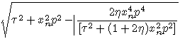
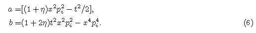
For non-hyperbolic curve approximation, we do not use the most accurate VTI equation. Though theaccuracy is higher, its complexity greatly increases and difficult to calculate. By weighing the accuracy and efficiencyof the computation, we choose Alkhalifah’s non-hyperbolic moveout equation(Alkhalifah and Tsvankin, 1995):

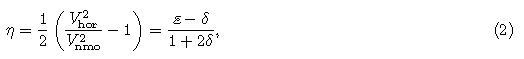
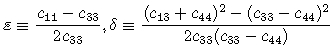 , cij is the elasticity coefficient( i, j = 1, 2, · · · 6).
2.2 Anisotropic Radon Transform
, cij is the elasticity coefficient( i, j = 1, 2, · · · 6).
2.2 Anisotropic Radon Transform
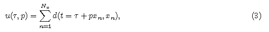
Discrete Linear Radon transform is defined as
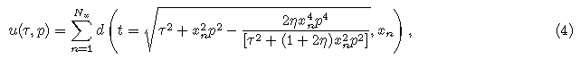
 is rewritten in the form of τ, the reverse anisotropic Radontransformation equation as
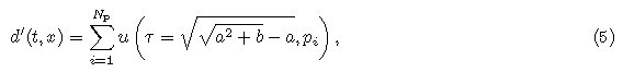
The formula of the anisotropic Radon transform is more complex because the equation of two parameters(offset x , slowness p )is replaced by the three-parameter equation(offset x , slowness p , η ). However, the processof the transform remains to integrate the curve to a point, and the matrix dimension of discrete computation issame. Therefore, the computational complexity of solution in time domain is similar to the hyperbolic Radontransform and other time-variable Radon transform. The accuracy of the non-hyperbolic integral depends onthe higher order offset and η .
2.3 The Discrete Equations of Anisotropic Radon TransformBased on the inversion theory, the Radon domain has higher resolution by first defining the inverse transform and then deriving the forward transform. The reverse anisotropic Radon transform Eq.(5)can be writtenin matrix form d' = Lm , where operator L is the reverse anisotropic Radon transform operator, and it is thematrix form of Eq.(4)defining the path of integration, and it means that a point in the Radon domain canbe transformed to a curve in the t-x domain controlled by x , p , and η . The forward operator LT of Radontransform means a curve in t-x domain controlled by t , p , and η can be transformed to a point in the Radondomain. By least-square inversion and weighting coefficient matrix Wm which improve the resolution of thesolution, the forward anisotropic Radon transform is defined as

It should be pointed out that the parameter η is not variable in the anisotropic Radon transform, eachdiscrete time t merely corresponds to one independent η , the accuracy of η is important to the accuracy of theanisotropic Radon transform. For the real seismic data, we should choose the best η and NMO velocity bydual-parameter velocity analysis method(Abbad et al. 2009). Those are the most distinct difference betweenthe anisotropic Radon transform and the other Radon transform. Although the anisotropic equation is morecomplex than conventional Radon transform, both of these transform computational processes are same. Theoperator matrix of tanisotropic and time-varying Radon transform has the same dimension.
2.4 The Optimal Semblance Weighting Gauss-Seidel AlgorithmIn order to get higher resolution of anisotropic Radon transform, the semblance weighting function isintroduced as
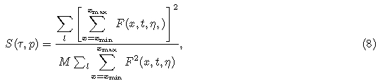

In Eq.(7)the operator L and LT is not time-varying, it can’t be solved in frequency domain. Basedon industrial high-resolution method on the Bayesian principle proposed by Sachhi, the calculation of sparseconstraintneeds several iterations and the conjugate gradient algorithm which is the most ordinary methodto implement Radon transform also needs lots of iterations, so the amount of computation is huge and theuncompressed operator matrix dimension is (nt×nx)×(nτ ×np) . Hence, the computation complexity increasesextremely with the increase of the seismic data dimension.
In order to decrease computation complexity, we adopt optimal Gauss-Seidel iterative algorithm with thesemblance weighting function Eq.(8)in anisotropic Radon transform. In this algorithm the result of previoustransform is used as priori information, the p-value s are ordered according to the semblance weighting functionvalues, the most significant integral energy of the p-value is first calculated and subtracted from t-x domain, and it loops all the sorted p-value and updates the results continually in the Radon domain. While calculatingthe p-trajectory, the energy in t-x domain continuallyattenuates until all the p-value calculation is completed.This algorithm emphasizes the initial p-value trajectory to ensure that the most significant initial p-value is involved in the overlay calculation, so thestrongest energy would be included in this path and a convergent result is achieved in the Radon domain.It takes a few iterations in this algorithm to get highresolution, so it can save much more computation.
The workflow of the anisotropic Radon transformwith optimal semblance weighting Gauss-Seideliterative algorithm is shown in Fig. 1. The semblanceweighting function is defined by non-hyperbolic moveoutcurve(Eq.(9)).

|
Fig. 1 Flowchart of the anisotropic Radon transform with semblance weighting Gauss-Seidel algorithm |
Step one: Calculate current slowness pi semblanceweighting function value and Radon domainresults uest(τ, pi) , and accumulate the values to the uacc(τ, pi) ;
Step two: Do inverse transform of uacc(τ, pi) to obtain dacc , original data d minus dacc to obtain d' , take d' as input data, repeat the step one by 3~5times iterative calculation, remaining energy can bereduced to an acceptable level in t-x domain, completeone slowness pi calculation;
Step three: Repeat the process of step one and step two to cumulate all the pi -value trajectory energyto uacc(τ, pi) , and constitute the final result of Radondomain.
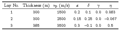
3 MODEL DATA AND FIELD DATA TEST 3.1 Anisotropic Media ModelIn this section, we establish a VTI anisotropic media model and its parameters are shown in Table 1. Thenumerical simulation data is 200 traces with 0~4000 m offset, it is processed by the parabolic, hyperbolic and anisotropic Radon forward transform respectively, the results are shown in Fig. 2, the Fig. 2a shows the shotrecord for the VTI media, zero offset t0 of primary reflection are 0.4 s, 0.64 s, 0.86 s, zero-offset t0 of multipleare 0.8 s, 1.2 s, 1.28 s, 1.72 s, 1.92 s; Fig. 2b shows the parabolic Radon transform result, the energy is obviouslynot convergent and has the phenomenon of dispersing and smearing; Fig. 2c shows hyperbolic Radon transformresult, it is better than Fig. 2b but the energy group is still not convergent, and both sides of the centre positionenergy contain a certain amount of energy extending; Fig. 2d shows anisotropic Radon transform result withthe highest resolution, the convergence of the energy is almost the same as the wavelet in simulation. Set thewhite cutting line as shown in Fig. 2d, the primary’s energy is above the line and the multiple’s energy is belowthe line. Fig. 2e shows the results of demultiple and Fig. 2f shows the multiples to be subtracted. By comparingthe computational efficiency of parabolic, hyperbolic and anisotropic Radon transform, the computational timeof the three transforms are 1.2 s, 8.5 s, 9.1 s respectively with Intel Core2 CPU of 2 Ghz clock and IntelC++ Compiler XE 12.1.2.278 parallel compiler. The anisotropic Radon transform’s computational efficiency isslightly higher than that of the hyperbolic Radon transform.
|
|
Table 1 Table 1 Parameters of the anisotropic model |

|
Fig. 2 Results of Radon domain of the anisotropic model (a) Simulated data of the VTI model; (b) Result of parabolic Radon transform; (c) Result of hyperbolic Radon transform; (d) Result of anisotropic Radon transform; (e) Primary gather; (f) Multiples gather. |
For the Radon transform is a non-orthogonal transform, the original signal can be approximately restoredbased on the least squares inversion algorithm. In order to compare the quantitative amplitude distortions ofthe parabolic, the hyperbolic and the anisotropic Radon transform, the Eq.(10)is given as
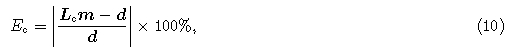
Figure 4a shows the gather of the marine seismic data, the sampling interval is 2 ms, record length is 12 s, the maximum offset is 8287 m. The reflection travel time curve is non-hyperbolic, especially when the ratioof offset to depth is greater than 1. The primary reflection below 3 s is almost suppressed by the multiple.Therefore, it is hard to restore the deep restructure from this field data. The red arrows indicate the primary and the black arrows indicate the multiple.

|
Fig. 3 Curve of η by dual-parameter velocity analysis and interpolation |

|
Fig. 4 Demultiple example of large offset marine data (a) Original gather with the maximum offset of 8287 m; (b) Result of hyperbolic Radon transform; (c) Result of anisotropic Radon transform and cutting line; (d) Zoom of the white frame of (b); (e) Zoom of the white frame of (c); (f) Primary reflection after demultiple of hyperbolic Radon transform; (g) Primary reflection after demultiple of anisotropic Radon transform; (h) Zoom of the white frame of (a); (i) Zoom in on the white frame of (f); (j) Zoom of the white frame of (g). |
For the real marine gathers, first step is acquisition of NMO velocity and anellipticity η by means ofthe dual-parameter velocity analysis. The numbers of η is equal to the numbers of picked seismic events.Therefore, we should linearly interpolate parameter η along the time direction, so that each discrete timesampling corresponds to one value of η . Fig. 3 shows the η parameter curve after interpolation. It should benoted that the correctness of η greatly impacts the resolution of anisotropic Radon transform, and the errorof η can lead to the incorrectness of the non-hyperbolic moveout travel time and reduce the resolution of thetransform, so several iterative processes of dual-parameter velocity analysis should be taken until the accurateparameter η is obtained.
The result of hyperbolic and anisotropic Radon transform is shown in Figs. 4b and 4c respectively, theenergy convergence of the latter is better than the former’s. By means of the optimal semblance weightingfunction Gauss-Seidel algorithm, the primary reflection and the multiple are separated obviously by the highresolution in anisotropic Radon domain. Figs. 4d and 4e are the zoom regions of the white frame in Figs. 4b and 4c. It is easy to set the red cutting line shown inFigs. 4b and 4c, the result of reverse hyperbolic and anisotropic Radon transform is shown in Figs. 4f and 4g, respectively. Compared with the original data, themultiple is suppressed well and there is little energyloss of the primary reflection at large offset. Then, theS/N ratio of the seismic gather is greatly improved.Figs. 4h, 4i, 4j are the zoom regions of the white framein Figs. 4a, 4f, 4g. Comparing the details of demultiple, both hyperbolic and anisotropic Radon transform perform well, but the latter can reserve more primary thanthe former.
Figures 5a, 5b show the velocity stack spectrum of the original gather and the result after anisotropicRadon transform, respectively. The former shows the obvious multiple at the velocity 1500 m/s as regular and equitable-time appearance of energy group along the timeline. The latter can be clearly distinguished that themultiple energy groups in Fig. 5a have been removed in Fig. 5b after the anisotropic Radon transform. Hencethe spectrum energy is relatively enhanced at the high velocity and at deep strata, it is the important evidenceof the demultiple effect.

|
Fig. 5 Comparison of velocity spectra (a) Velocity spectrum of original gather; (b) Velocity spectrum of primary after anisotropic Radon transform demultiple. |
By adding the anisotropic parameter in integral path of Radon transform, we get the anisotropic Radontransform which is defined by three parameters, i.e., the offset x, the slowness p, and the anellipticity η .We derive the forward and reverse formula of anisotropic Radon transform and adopt the optimal semblanceweighting Gauss-Seidel iterative algorithm to achieve high resolution in Radon domain. It can avoid largematrix operations in time domain, so our method maintains high computational efficiency.
The parameter η should be obtained by dual-parameter velocity analysis before the anisotropic Radontransform. For each discrete time, it requires one corresponding η . The value of η greatly influences theresolution of anisotropic Radon domain, so the correct η in accordance with optimal NMO velocity should bechosen.
The resolution of Radon domain for the large offset marine data is significantly improved after anisotropicRadon transform. In spite of small moveout, the primary reflection and multiple can be separated clearly. The result retains effective reflection information of large offset that is essential to the imaging of steep and deepstructure.
This work was supported by the National Natural Science Foundation of China(41204078).
| [1] | Abbad B, Ursin B, Rappin D. 2009. Automatic nonhyperbolic velocity analysis. Geophysics, 74(2):U1-U12. |
| [2] | Alkhalifah T, Tsvankin I. 1995. Velocity analysis for transversely isotropic media. Geophysics, 60(5):1550-1566. |
| [3] | Beylkin G. 1987. Discrete radon transform. IEEE Transactions on Acoustics, Speech, and Signal Processing, 35(2):162-712. |
| [4] | Feng X, Zhang X W, Liu C, et al. 2011. Separating P-P and P-SV wave by parabolic Radon transform with multiple coherence. Chinese J. Geophys. (in Chinese), 54(2):304-309, doi:10.3969/j.issn.0001-5733.2011.02.005. |
| [5] | Gong X B, Han L G, Wang E L, et al. 2009. Denoising via high resolution Radon transform. Journal of Jilin University(Earth Science Edition) (in Chinese), 39(1):152-157. |
| [6] | Gong X B, Lv Q T, Han L G. 2013. Anisotropic Radon transform.//75th EAGE Conference & Exhibition Extended Abstracts. |
| [7] | Huang X W, Wu L, Song W. 2004. 3D Pre-Stack depth migration with radon projection. Chinese J. Geophys. (in Chinese), 47(2):321-326. |
| [8] | High resolution Radon transform in the t-x domain using "intelligent" prioritization of the Gauss-Seidel estimation sequence.//74th Ann. Internat Mtg., Soc. Expi. Geophys. Expanded Abstracts, 2160-2163. |
| [9] | Niu B H, Sun C Y, Zhang Z J, et al. 2001. Polynomial Radon transform. Chinese J. Geophys. (in Chinese), 44(2):263-271. |
| [10] | Pan D M, Hu M S, Cui R F, et al. 2010. Dispersion analysis of Rayleigh surface waves and application based on Radon transform. Chinese J. Geophys. (in Chinese), 53(11):2760-2766, doi:10.3969/j.issn.0001-5733.2010.11.025. |
| [11] | Sacchi M D, Ulrych T J. 1995. High-resolution velocity gathers and offset space reconstruction. Geophysics, 60(4):1169-1177. |
| [12] | Schonewille M A, Aaron P A. 2007. Applications of time-domain high-resolution Radon demultiple.//77th Ann. Internat Mtg., SEG Technical Program Expanded Abstracts, 2565-2569. |
| [13] | Trad D O, Ulrych T J, Sacchi M D. 2002. Accurate interpolation with high-resolution time-variant Radon transforms.Geophysics, 67(2):644-656. |
| [14] | Wang J F, Ng M, Perz M. 2010. Seismic data interpolation by greedy local Radon transform. Geophysics, 75(6):WB225-WB234. |
| [15] | Wang W H, Shou H, Liu H, et al. 2006. High resolution τ-ρ transform in linear events wavefield separation. Progress in Geophysics (in Chinese), 21(1):74-78. |
| [16] | Wang W H, Pei J Y, Zhang J F. 2007. Prestack seismic data reconstruction using weighted parabolic Radon transform.Chinese J. Geophys. (in Chinese), 50(3):851-859. |
| [17] | Wang Y H. 2003. Multiple attenuation:Coping with the spatial truncation effect in the Radon transform domain.Geophysical Prospecting, 51(1):75-87. |
| [18] | Xiong D, Zhao W, Zhang J F. 2009. Hybrid-domain high-resolution parabolic Radon transform and its application to demultiple. Chinese J. Geophys. (in Chinese), 52(4):1068-1077. |
| [19] | Zeng Y L, Le Y S, Shan Q T, et al. 2007. VSP wavefield separation based on high-resolution Radon transformation.Geophysical Prospecting for Petroleum (in Chinese), 46(2):115-119, 173. |