1 INTRODUCTION

Full waveform inversion(FWI)makes full use of the observed seismic records to obtain the elastic propertiesof the subsurface media(Pica et al ., 1990). The purpose is to find a model whose synthetics can optimally matchthe observed data. Because of the full use of information contained in the waveform, FWI can greatly improvethe inversion resolution and accuracy compared with the traditional traveltime tomography(Tarantolla, 1984;Zhou and Gerard, 1993). Since the 1980s, many studies have focused on the waveform inversion based on theleast-square objective function(Woodward, 1992; Devanvey, 1984; Wu and Toksoz, 1987; Pratt and Goulty, 1991; Schuster and Aksel, 1993). Tarantola(1984)proposed that the gradient of this objective function canbe calculated by cross correlation of the forward wavefield from the sources and the back propagated wavefieldof the residuals from the receivers. This achievement pushed its development. Mora(1987)developed FWIto elastic media in theory. Zhou and Gerard(1993), Pratt et al .(1998) and Wu et al .(2006)applied FWIto borehole imaging successfully. Pratt et al .(1998)proposed an approach to implement FWI in frequencydomain, which makes FWI possible to be applied to field data. Recently, the adjoint-state method derived from Tarantola(1984)has become a regular approach to calculate the gradient of variable objective function withvariable state equation(Plessix, 2006).

An accurate near-surface velocity model is important for static correction, datum continuation and topographicmigration. Traditional ray-based first-arrival traveltime tomography(RFTT)is widely used to buildthe near-surface velocity model, but the obtained results usually lack short-wavelength components dues to thehigh-frequency approximation of ray theory. Liu et al .(2009)proposed the Fresnel volume tomography(FVT)based on finite-frequency theory(Dahlen et al ., 2000)to reveal both long- and short- wavelength componentsof the near-surface velocity model. The sensitivity kernels of FVT are derived from the wave equation, and the traveltime of the main energy of the seismic wave is used, thus it can achieve better results than RFTT inboth synthetic tests and field data processing. Bae et al .(2012)compared the sensitivity kernels of FVT and Laplace FWI, and pointed out that Laplace FWI can reveal deeper structures than FVT even it is still using thefirst-arrival traveltime. Sheng et al .(2006)showed that the first-arrival waveform contains little informationof the deep structure, but it can be used to reconstruct the fine near-surface velocity structure. They alsoindicated that first-arrival waveform inversion(FAWI)has a weaker dependence on the starting model thantraditional FWI for its relatively good linearity and stability. However, Sheng et al .(2006)used the dampedwave equation to simulate the first-arrival waveform, which doesn’t decrease the forward computation at allcompared with the traditional FWI.

FWI is computationally expensive due to the forward modeling in each iteration. Liu(2011)used theGaussian beam(GB)to simulate the Green function and the(first-arrival)synthetics with high efficiency.Therefore, to improve the efficiency of FAWI, we use the GB as the forward modeling approach in this paper.The subsequent problem is that it’s hard to use the adjoint-state method to calculate the direction and the steplength of the objective function if GB is involved. Woodward(1992)gave two sensitivity kernels based on Born and Rytov approximations respectively of acoustic wave equation. He called them Born wavepath and Rytovwavepath. Up to now, these kernels are successfully applied to wave-equation tomography, finite-frequencytomography(Dahlen et al ., 2000) and FVT(Spetzler and Snieder, 2004; Liu et al ., 2009). But due to the hugestorage, the sensitivity kernels are seldom used in FWI. In this paper, we propose a rapid matrix-decompositionalgorithm to deal with the kernel-vector product to calculate the direction and the step length, through whichthe storage of the whole kernels is not necessary any more.

We call this method as Gaussian beam first-arrival waveform inversion(GBFAWI)based on Born wavepath.The applications of this method, traditional FWI and RFTT to synthetic tests show that GBFAWI can reconstructthe fine near-surface velocity structure without losing efficiency.

2 INVERSION METHOD

In waveform inversion, the objective function is usually defined as

where v is velocity, u_o indicates the observed data, u_c is the synthetics satisfying the acoustic wave equation.The purpose of the above inverse problem is to find a solution v⁺ which minimizes the objective function.

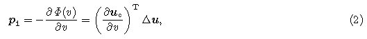
According to the optimization theory, an iteration theme is usually used to solve the above inverse problem.In each iteration, the update of the velocity △v can be expressed as the product of the direction vector p and the step length t. Direction p can be obtained by solving the gradient of the objective function directly orindirectly. The following directions and step lengths are regularly used

where p₁ and p₂ are the first-order and second-order directions respectively, and p can be either p₁ or p₂ . p₂ and p₂ are the corresponding step lengths. △u = u_o ? u_c is the wavefield residual. H_a which is called Hessianmatrix is the approximate second-order derivatives of the objective function Φ(v) with respect to the modelparameters. аu_c / аv is the Fr′echet derivative or the sensitivity kernel which shows the influence of velocityperturbation on the wavefield variation. Upper T means the conjugate transpose of a complex matrix.

It’s quite hard to directly calculate any direction or step length according to the above equations becauseboth Frchet derivative and Hessian matrix are difficult to be achieved. Woodward(1992)gave the relationshipbetween wavefield variation of a source-receiver pair(g, s) and velocity perturbation based on the Bornapproximation of the acoustic wave equation

where g denotes the receiver position, s indicates the source position, r is an arbitrary position in space. v₀ indicates the media without perturbation, and △v is the perturbation of v₀ . G₀(g, r) is the Green functionat point g from a source r under unperturbed media, and u₀(r, s) is that at point r from a source s. Notethat Born approximation belongs to the first-order approximation, hence it cannot describe the higher-orderscattering caused by an anomaly. Therefore, a good starting model is needed for FWI to iteratively reach thenonlinear relationship between media and wavefield.

It’s easy to get the kernel function which expresses the first-order linear relationship between wavefieldvariation and velocity perturbation

Substituting Eq.(7)into(2), we get

And then Eqs.(2)–(5)can be rewritten as

If the data has m elements and the model consists of n discrete parameters, the dimensions of the direction p is n × 1, that of △u is m × 1, and that of K is m × n. It’s easy to see that in practice the matrix K ishard to be stored, hence the direct calculation of p₁ or p₂ is almost impossible. However, Virieux and Operto(2009)realized the indirect calculation of the gradient of the objective function using the adjoint-state method(Plessix, 2006)

where u^t indicates the forward wavefield, аA/аv is called the radiation pattern, A^?1 △u ⁺ is the back propagatedwavefield of the residual, and upper + denotes the conjugate operator. By this way, the computation and storageof matrix K is avoided. At present, the adjoint-state method has become the regular approach to calculate thedirections of FWI.

3 GAUSSIAN BEAM SIMULATION OF THE FIRST-ARRIVAL WAVEFIELD

First-arrival waveform can be inverted for the fine near-surface velocity structure. Meanwhile, FAWI isless dependent on the starting model, more linear and more stable than traditional FWI(Sheng et al ., 2006).However, forward simulations are needed in each iterative in waveform inversion. To reduce the computation, we use the Gaussian beam to realize the rapid calculation of the first-arrival wavefield and the Green function.Gaussian beam is based on the high-frequency asymptotic approximation, whose accuracy can only be guaranteedwhen the frequency is high. The error increases when the frequency decreases, but it’s still reasonable to useGaussian beam to calculate the wavefield and the Green function under certain accessible inversion resolution(Zhao et al ., 2012).

Since the Gaussian beam is the asymptotic solution of the elastic equation near the central raypath, italso represents the high-frequency Green function in the same area. To get the Green function on the paraxialray as well as the central ray, we use the equation given by Zhao et al .(2012)

where T(s) is the traveltime of the seismic wave along the central raypath, vector q is the paraxial coordinateunder the ray-center coordinates, s is the arc length from the starting point, and M(s)is the second-orderpartial derivative of the traveltime field with respect to the spatial coordinates.

To prove the effectiveness of the Gaussian beam method on forward modeling, we simulate the wavefieldin a numerical model which is discretized by a 201×201 grid with grid interval being 25 m ×25 m. Thehomogeneous velocity is 3500 m·s^-1. The synthetics are shown in Figs. 1 and 2.

4 COMPUTATIONS OF DIRECTION AND STEP LENGTH

We use the Gaussian beam to simulate the wavefield and Green function, thus it’s difficult to calculate thegradient of the objective function of FAWI using the adjoint-state method. Therefore, we calculate them directlyusing Eqs.(10)–(13). To improve the computation efficiency and reduce the memory storage, we propose thefollowing matrix-decomposition realization of the kernel-vector product, once we have got the Born wavepath, to implement the calculations of the directions and the step lengths.

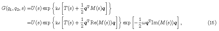
Once G0(r, g) and u₀(r, s) are achieved by the Gaussian beam method, the first-order direction p₁ canbe obtained by Eqs.(7) and (10)through matrix decomposition as shown in Eq.(16). After decompositionevery column in K^T (marked by the rectangle)has the specific physical meaning of being the conjugate of thesensitivity kernel of a certain source-receiver pair. Therefore, it’s not necessary to store the whole kernel matrix K beforeh and . Only one sensitivity kernel is needed to be calculated and stored in memory at any time, and then the direction p₁ can be obtained through accumulation. By this way, not only the storage is greatly savedbut the inversion scheme proposed by Woodward(1992)can be put into practice.

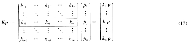
In the same way, the computation of KP in p₂ can be accomplished by row decomposition as shown inEq.(17). Note that each row in kernel matrix K (marked by the rectangle)is the sensitivity kernel of a certainsource-receiver pair.

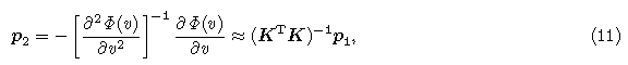
In theory, the calculation of the second-order direction p₂ is much more difficult. At present, the L-BFGSmethod(Nocedal, 1980)is widely used to compute it approximately, but the error is huge in some conditions.M′etivier et al .(2012)gave an algorithm to iteratively construct p₂ in an extra inner loop, but two forwardsimulations are needed in each iteration of the inner loop, thus the computation is greatly increased. Usingthe matrix decomposition proposed in this paper, we can also iteratively construct p₂ while without needingto do forward simulation any more. The detailed procedure will be given in another paper. Considering thatthe diagonal components in Hessian matrix are dominant, the diagonal Hessian is widely used now to constructthe second-order direction p₂ . Correspondingly, this direction is called diagonal pseudo Newton(Choi and Shin, 2007). Physically, these diagonal components denote the illumination of the acquisition on the subsurfacemedia. Therefore, it’s not difficult to underst and through Eq.(3)or(11)that such a way is indeed a kind ofillumination compensation to the first-order direction, thus this implement is also known as preconditioning ofthe first-order direction. Using the matrix decomposition approach, we can also realize the computation of suchan approximate diagonal Hessian H_a as shown below,

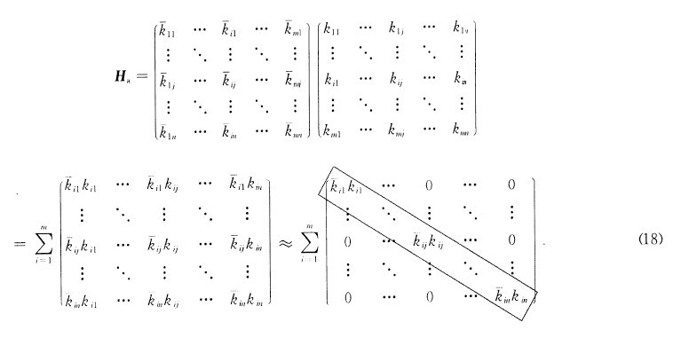
In the above equation, every diagonal matrix on the right side can be calculated according to the correspondingsensitivity kernel(marked by the rectangle)of a certain source-receiver pair. Thus, we don’t need tocalculate or store the whole kernel matrix K beforeh and either. Only one sensitivity kernel is needed to becomputed and stored at any time, and then H_a can be obtained by accumulation. After substituting H_a intoEq.(3)or(11), we get the diagonal pseudo Newton.

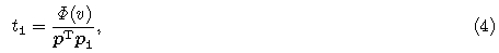
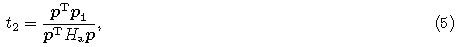
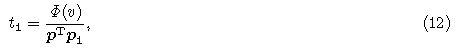
Once the first-order direction p₁ or the second-order direction p₂ is constructed, the computation of thecorresponding step length t₁ or t₂ is straightforward using Eq.(12)or(13)respectively.

5 SYNTHETIC TESTS

To test the effectiveness of the proposed method, we compare it with RFTT and traditional frequencydomainacoustic FWI on the 2D Inclusion 1 model(Operto et al ., 2007). The real model is shown in Fig. 3, which consists of 201×201 nodes with node interval being 25 m×25 m. The background velocity is 3500 m·s^-1, and the anomaly velocity is 3700 m·s^-1. 84 sources and 84 receivers are uniformly spread on the four sides 500 minner from the edges. Both source interval and receiver interval are 200 m. The two waveform inversions use thefirst-order direction and the first-order step length. 10 frequencies are inverted with the starting frequency being2 Hz, and the frequency interval being 2 Hz as well. 10 iterations are implemented for each frequency. RFTTis not related with frequency, and the iteration number is set to be 20 for convenient comparison. The startingmodels for the three methods are the same being homogeneous background velocity. The final reconstructedresults are shown in Figs. 4–6. To compare the results quantitatively, a horizontal profile at z=2500 m and avertical profile at x=2500 m are extracted as shown in Fig. 7.

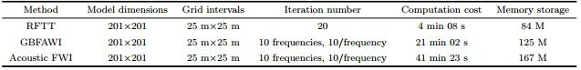
From Figs. 3–7 we can see that all of the three methods obtain good results because the model is simple and well covered by the acquisition. Meanwhile, it’s not difficult to find that the accuracy and resolution of theresult of GBFAWI is a little lower than traditional FWI, while much higher than RFTT. This is because that GBFAWI makes use of the first-arrival waveform instead of just the traveltime, and it uses the Gaussian beammethod to simulate the wavefield instead of the wave equation. The computation efficiencies and memory storagesof the three methods are shown in Table 1, from which we can find the big advantage of GBFAWI. Note that, similar with traditional frequency-domain FWI, the computation cost of frequency-domain FAWI is positivelyproportional to the inverted frequencies and the iteration number for each frequency. Thus, after normalizingthe iterations of RFTT and GBFAWI we can find that they have the similar efficiency in computation.

To test the capability of GBFAWI on complex models, we compare it with RFTT and FWI through theOverthrust model(Operto et al ., 2007). The real model is shown in Fig. 8, which is discretized by an 801×187 grid with grid interval being 25 m×25 m. 199 sources are distributed at 25 m below the surface uniformly, with the interval being 100 m. 200 receivers spread on the surface with interval of 100 m. The first sourcelocates at 50 m in horizontal direction, and the first receiver locates at 25 m. To increase the inversion accuracy and convergence rate, we use the second-order direction and step length in the two waveform inversions. 10frequencies are used, and the starting frequency is 2 Hz, with the interval being 2 Hz as well. 10 iterations areperformed for each frequency. The RFTT is not related with frequency, thus the iteration number is set to be 20for convenient comparison. The starting models shown in Fig. 9 are the same which is constructed by Gaussiansmoothing of the real model. The revealed results are shown in Figs. 10–12. To compare them quantitatively, the horizontal profiles at 500 m, 750 m, and 1000 m in depth are extracted in Fig. 13.

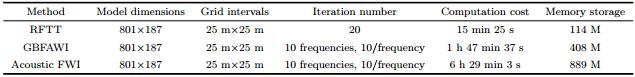
Through comparisons of Figs. 8 and 10–13, we find that GBFAWI can reconstruct the fine near-surfacevelocity structure of the complex model. Because only the first-arrival waveform is used in GBFAWI the shallowreconstruction is a little worse than the traditional acoustic FWI, and the deep parts are much worse. However, compared with RFTT the shallow reconstruction of GBFAWI is much better, and deeper parts are revealed.Through Table 2 we can find again that the computation cost of GBFAWI doesn’t increase a lot compared withRFTT. From the convergent curves as shown in Fig. 14, we can see that GBFAWI is stable, even better thantraditional FWI in the high-frequency b and .

Due to that only the first-arrival waveform is used, FAWI has a weaker dependence on the starting modelcompared with conventional FWI(Sheng et al ., 2006). This is another advantage of the proposed GBFAWI. Totest this, we construct another starting model(as shown in Fig. 15)got by large-scale Gaussian smoothing ofthe real Overthrust model. Obviously, this starting model is almost 1D gradient. The reconstructed results of GBFAWI and traditional FWI are shown in Figs. 16 and 17, and the horizontal velocities at 500 m belowthe surface are shown in Fig. 18. We can see that the traditional acoustic FWI quickly converges to a localminimum which is far away from the real one. However, the result of GBFAWI still has good vertical and horizontal resolutions at the shallow parts, though the accuracy decreases compared with Fig. 11.

6 CONCLUSIONS

We propose a Gaussian beam first-arrival waveform inversion approach based on the Born wavepath. Thismethod inverts the first-arrival waveform for the near-surface velocity structure. In the forward modeling, theGaussian beam is used to simulate the Green function and spatial wavefield with a high efficiency. In theinversion part, we give a matrix-decomposition algorithm based on the Born wavepath to deal with the kernelvectorproduct to decrease the memory storage. Synthetic tests show that the proposed GBFAWI can not onlyachieve a much finer and deeper velocity model than RFTT without increasing the computation much, butalso the revealed result keeps the similar quality as the traditional FWI at the shallow parts. Meanwhile, thismethod has advantages of high efficiency, small memorial storage, strong stability and weak dependence on thestarting model. It can be easily exp and ed to 3D to show its great potential to process the field data.

This work was supported by the National Natural Science Foundation of China(41274116).