 2014, Vol. 57


2. The Second Institute of Oceanography, State Oceanic Administration, Hangzhou 310012, China
The South China Sea(SCS)is a special continental marginal sea, containing a lot of signals about seafloor spreading and the formation of the sea basin(Li et al., 2011). The crustal structures from seismic reflection/ refraction experiments are relatively reliable and can present direct proofs for the conjugation relationship of the separated margins of the SCS. The ocean bottom seismometers(OBS)lines in the SCS are mainly distributed on the northern margin and fewer on the southern margin(Fig. 1)(Qiu et al., 2011). The wide angle seismic profile OBS973-2, crossing northeastern Reed Bank and extending to the sea basin, has important significances for underst and ing the conjugate crustal structure of the SCS(Qiu et al., 2011; Ruan et al., 2011).

|
Fig.1 Map showing water depth and deep seismic profiles in the South China Sea. The profiles of this study are marked in red (OBS973-2) and yellow (NH973-2), respectively. The left inset is the OBS line location of this study, the white circles represent the OBS recovered and the red circles represent OBS lost |
Ruan et al.,(2011)have simulated the P-wave velocity structure of profile OBS973-2, showed much more similarity with that of profile OBS2006-1 in the western section of the northern margin and supposed Reed Bank and Macclesfield to be a pair of conjugate blocks. However, the previous model lacks inversion fitting errors calculation and model uncertainties and resolution estimation due to limitation of the software WARRPI they used(Ditmar and Makirs, 1996). Moreover, the multi-channel seismic(MCS)profile NH973-2(Ding and Li, 2011)parallel close to OBS973-2(at distance of 2~3 km)should be used to constrain crustal structures. Although both MCS data and OBS data have been used for the study of crustal structures of the SCS, the former is more often used for shallow structure(Song et al., 2001; Xu et al, 2006; Ding and Li, 2011); the latter is used to simulate the deep crust and rifting deformation structures of marginal seas(Yan et al., 2001; Ruan et al., 2004, 2011; Zhao et al., 2010; Wu et al., 2010; Hao and You, 2011; Qiu et al., 2011; Huang et al., 2011; Wei et al., 2011a, b). Therefore, we intend to use the forward simulation technique(Zelt and Smith, 1992) and trial- and -error or automatic inversion method(Hobro et al., 2003)to remodel profile OBS973-2, combined with MCS data of NH973-2. The data of MCS are used to constrain the shallow interfaces in the OBS model and the velocity distribution derived from wide-angle seismic data are used in the time-depth conversion of MCS data simultaneously. By such mutual constraint, we establish three models: refraction forward model, automatic inversion model and geological interpretation model from MCS. Finally we compare and combine these three models together to construct the fine P-wave velocity structures of Reed Bank and the adjacent sea basin and to reveal dynamic characteristics at depth.
2 OBS DATAThe wide angle seismic profile OBS973-2 that extends in NW-SE direction for 369 km crosses the northeastern Reed Bank and reaches the central sub-basin(Fig. 1). Seventeen OBS were deployed along the profile in 20 km interval(OBS1 and OBS10 were lost). The seismic experiment, data acquisition and data processing have been illustrated in detail by Ruan et al.(2011).
The seismic data of fifteen OBS used in this work is of high quality in general and contains various deep signals(Fig. 2). All stations recorded direct water waves Pw, refraction waves from the upper crust Pg1(Watremez et al., 2011), most stations recorded reflection waves of the Moho PmP and refraction waves from the upper mantle Pn, and some stations recorded refraction signals from the lower crust Pg2. The seismic signals can be traced to maximum offset of 120 km. In addition, the data of the MCS NH973-2, parallel to OBS973-2 with distance of 3 km completed by R/V “Tan Bao” in 2009(Fig. 1), and its geological interpretation(Ding and Li, 2011)can be used to offer some constrains on shallow structure in the simulation profile OBS973-2.

|
Fig.2 Seismic section of OBS3 station on OBS973-2 profile (reduced velocity of 6 km/s) |
We construct a starting model based on the MCS profile, regional geophysical and geological data and previous work, and analyze and identify seismic phases presented in the OBS seismic sections. Then we use 2-D ray-tracing method to simulate synthetic travel times of all kinds of phases, fit them with observed arrivals by a trial- and -error approach and modify some parameters of the model until we achieve the optimum P-wave velocity model that has the minimum fitting error(root mean square misfits, RMS). Finally we calculate synthetic ray paths of the optimum model from sediment to mantle. Here we use software of RayInvr(Zelt and Smith, 1992)for all calculations mentioned above.
Based on the previous model of the same OBS line(Ruan et al., 2011) and seismic phases in seismograms, we identify and pick various seismic phases and calculate their ray paths in modeling stages. For example, OBS8 station, located in COT section along the OBS line, presents Pg1 and PmP with maximum offset of 60 km in its right branch. In its left branch(corresponding to sea basin)Pg1, PmP and Pn are identified with maximum offset of 80 km(Fig. 3a). The results of its ray-tracing and travel times fitting are all very well(Fig. 3b, and 3c). We combine ray-tracing results of all stations to constrain the velocity model, and then conduct repeated simulation until we achieve the optimum 2D model and ray density coverage(Fig. 4). We use the fitting errors RMS and the chi-squared(χ2)value(optimum 1.0)to weigh the mismatch between the observed and calculated arrival times(Zelt and Smith, 1992) and calculate rays coverage to estimate the reliability of the model. Furthermore, we conduct checkerboard tests to estimate data quality and recovering ability. We suppose seismic phases picking associated uncertainties to be ±50 ~ ±80 ms based on estimation of data quality.

|
Fig.3 (a) Seismic section of vertical component of OBS 8; (b) Simulation of ray-tracing; (c) The fitting of the calculated travel time to observed |
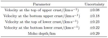
The P-wave modeling shows that the travel time RMS are small in general with a little bit increasing downward and the maximum RMS is less than 120 ms. The χ2 values are within 1.1~1.9 indicating well fitted(Table 1). The ray coverage shows that the main crustal layers and upper mantle in the final model(Fig. 4a)are well covered 10~40 times(minimum of 5), indicating high reliability and resolution of the model. The perturbation test of interfaces and velocities(Zelt and Smith, 1992; Muller et al., 1997)shows that the uncertainties of crust velocity and Moho depth are < 0.25 km/s and ±0.29 km, respectively(Table 2).
| Table 1 Picks and rays simulation of profile OBS973-2 |

| Table 2 Uncertainty analysis of model parameters |

|
Fig.4
(a) Crustal velocity structure of profile OBS973-2 from forward modeling; (b) The distribution
of rays density with the size of statistic network: 0.5 km×0.25 km V.E.=5. The black circles with numbers are OBS positions. The white lines with numbers are the positions of 1D velocity curves discussed later. |
We also use the Jive3D code(Hobro, 1999; Hobro et al., 2003)for modeling crustal structure of the same OBS profile, since its technique can be used not only in forward simulation but also in tomographic inversion. The velocities and depth are presented by regular grid nodes and fitting algorithm allows travel time misfit error and model complexity to be reduced to minimum simultaneously and to achieve simplest structures in 1D, 2D and 3D. The data of wide-angle reflection or refraction and of large offset MCS can be combined in the inversion process(Hobro, 1999). The target function of simulation is defined as

Since only 2D model structure is simulated, one horizontal dimensional size is kept as 1 in Jive3D code(Hobro, 1999) and back-stripping scheme(Paulatto et al. 2010)is used to keep suitable constrains on interfaces and layers when depth increases. In one inversion stage the present layer and interfaces above it are all simulated. Before conducting inversion exercise seismic phases should be identified by some initial model and forward calculation, for automatic inversion is not directly visible(Paulatto et al, 2010). The P-wave velocity model obtained by repeated forward simulation in last stage is used here as a starting model for automatic inversion(Fig. 5a). The velocity field is assumed to be continuous and smooth in layers(sea water, crust and upper mantle)with crust velocity variation ranging from 1.8 km·s-1 to 7.0 km·s-1 and upper mantle velocity variation range from 8.0 km·s-1 to 8.2 km·s-1. The Moho discontinuity is designed as a simple tilting interface, and then interpolation algorithm is applied to the velocity field to form a homogeneous model presented by grid nodes(Fig. 5b). During inversion stages, two-time spline interpolation function(type B)is automatically used to form constant velocity gradients in the new grid and linear interfaces. The coarser of grid, the better for avoiding over fitting so long as the fitting accuracy is not influenced(Scott et al., 2009). The grid-node spacing is 5 km(horizontal)×0.5 km(vertical)for the model of 370 km in length and 30 km in depth. The number of velocity nodes is 76×3×62 in crust layer and 76×3×9 in upper mantle layer, and the number of grid nodes of seabed is 373 with interval of 1 km and 40 of Moho discontinuity with interval of 10 km, respectively. The discontinuities of the velocity field are attributed to interfaces and represented by smooth and continuous depth polynomial functions. The phases and their uncertainties used in automatic inversion are the same as that in forward simulation(Pg1 and Pg2 are combined as Pg), but without direct water waves. The value of parameter λm is gradually reduced from zero to -9.99 in interval of -0.2, and each λm should be alternatively changed eight times until a stable model is achieved, consequently the model optimization reduced from 30%(λm is Zero)to 0.001%(λm is the smallest), and χ2 is reduced from 884.01 to 1.11(Fig. 6). The final P-wave velocity(Fig. 5c), with phases fitting ratio >80%, which is close to the real geological one. We use the checkerboard method(Paulatto et al. 2010)to test the resolution of the model(Fig. 7), with velocity perturbation 5% and sinusoidal perturbation halfwavelength of 50 km×2 km. The test shows that the model simulated by automatic inversion has very good resolution in vertical direction and acceptable resolution in horizontal direction, for the end parts have not enough ray coverage.

|
Fig.5 Automatic inversion process and models in stages: initial model(a), parameterized simple model(b) and the final model(c)derived from automatic inversion approach. The others are the same as Fig. 4 |

|
Fig.6 Contour plots of inversion parameters |

|
Fig.7
Result from the checkerboard resolution test for inversion model Panel(a)shows perturbation added to the final model, and panel(b)shows recovered perturbation. A sinusoidal perturbation with half-wavelength of 50 km×2 km was tested. And the velocity perturbation contour is 0.5 km·s-1. The others are the same as Fig. 4. |
Time-Depth Conversion Based on Simulated OBS Velocity Model After amplitude compensation, static moveout, gain processing, deconvolution, elimination multiple waves, velocity analysis, residual static moveout and frequency analysis, the MCS profile NH973-2 has been completed by migration stacking, after stacking deconvolution and high frequency b and filtering(Ding and Li, 2011). We use the velocity distribution derived from automatic inversion of OBS line to convert the arrival times of MCS profile into depths, and finally obtain a new crustal structure model(Fig. 8). It shows that the three 2D models are generally in consistent with each other, but wide-angle seismic data constrain deep structures better.

|
Fig.8 Crustal structures of profile of NH973-2 (black) resulted from time-depth conversion in comparison with that of OBS973-2 from forward simulation (red) and automatic inversion (green) |
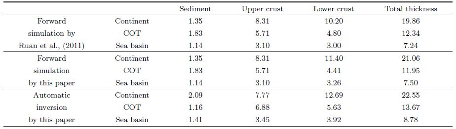
The model derived from interactive forward simulation(Fig. 4a)consists of seven layers, including sea water(velocity 1.5 km·s-1) and three sediment layers. The sediment layers are 1~2 km thick on average, lacking layer 2 and layer 3 in some sections along the OBS line with velocities downward increasing from 1.8 km·s-1 to 4.5 km·s-1. The upper crust has relatively large laterally variation of thickness from 3~4 km in sea basin, 5~7 km in the transition zone to 7~8 km at Reed Bank, and velocities downward increase from 5.0~5.5 km·s-1 to 6.4 km·s-1. The lower crust also has large laterally variations of thickness from 3~4 km in the sea basin, 4~5 km in the transition zone to 9~12 km at Reed Bank and velocities downward increase from 6.5 km·s-1 to 6.9~7.2 km·s-1. The velocity at the Moho discontinuity varies from 8.0 km·s-1 to 8.2 km·s-1 along the line(Table 3). On the other h and , the model derived from automatic inversion(Fig. 5c)comprises three layers: sea water, crust and upper mantle, showing similar layer thickness to that of other two models(Table 3 and Fig. 8). But the total crust thickness of the model derived from automatic inversion is 1.5 km larger than the others, because its Moho discontinuity lacks constraint of PmP phases and influenced by travel time uncertainty. However, such error is less than 5% of the total model depth(30 km). There is a high velocity zone in crust at model distance 120 km, and checkerboard perturbation recover is worse. Compared with forward simulation, automatic inversion shows good fitting(χ2 is 1.11, better than 1.643 of forward simulation) and high effectives, suggesting the automatic inversion method should be used when the data have enough constrains on interfaces.
| Table 3 Comparison of models from forward simulation and automatic inversion (average layer depth/km) |
The seabed in NH973-2 model(Fig. 8)is some different from that of OBS973-2 due to their uncompleted coincidence and distance of 3 km, but such difference has no influence on structure interpretation. The sediment basement in COT along NH973-2 is consistent with the velocity contour of 4.8 km·s-1 in the automatic inversion model deeper than that in the forward simulation model, indicating the sediment maximum velocity is less than 4.8 km·s-1 or the velocities used in time-depth conversion are smaller than they should be. The Moho depth along NH973-2, calculated by the average velocity in the range of 180~260 km, is highly in agreement with that in the other two models at distance 205~260 km, indicating that MCS can derive reliable deep structure by using the constraint from the automatic inversion model of OBS data.
The models presented in this paper are also highly consistent with that of previous study(Ruan et al., 2011), shown as Table 3. But we use χ2 to analyze model misfit errors(Table 1) and calculate model uncertainties(Table 2).
4.2 Reed Bank Crust Structure and Its Tectonic ImplicationsThe continental crust in the model section of 0~200 km is 21~23 km thick with velocity downward increasing from 5.5~5.8 km·s-1 to 6.9~7.2 km·s-1, and has abnormal laterally variation of velocity and a low velocity zone in the upper crust. The 1D velocity structures at distances 46 km, 72 km and 170 km(Fig. 9)all exhibit extensional marginal structure characteristics and indicate the presence of low velocity anomalies and velocity reversing. Correspondingly the same section in the MCS profile shows the presence of a series grabens cutting through basement even to lower crust(Fig. 8), indicating this region has experienced tectonic extension activities even until present(Ding and Li, 2011).

|
Fig.9
Comparison of continental crust 1D vertical velocity curves derived from forward simulation(red curve) and automatic inversion(green curve)with other settings (a)Vertical velocity in model 46 km, black envelope represents extended continental crust(Christensen and Mooney, 1995) and shadow zone represents average continental crust(Christensen and Mooney, 1995);(b)Vertical velocity in model 72 km, the others are same as Fig. 9a;(c)Vertical velocity in model 170 km, the others are same as Fig. 9a. |
The COT section(model distance 200~280 km)has a tinning crust 11~12 km derived from forward simulation(13~14 km derived from automatic inversion). The comparison of 1D velocity structures at distances 217 km, 240 km and 280 km(Fig. 10)with the serpentine velocity curves in drill ODP1277(Christensen and Mooney, 1995) and Atlantic COT(Sibuet and Tucholke, 2012), shows that the upper crust has a serpentine velocity and the lower crust has a little lower velocity than serpentine and without HVL, suggesting the southern margin of the SCS is a non-volcanic margin.

|
Fig.10
Comparison of COT crust 1D vertical velocity curves derived from forward simulation(red curve) and automatic inversion(green curve)with other settings (a)Vertical velocity in model 72 km, black line represents serpentine velocity from ODP1277 site(Sibuet and Tucholke, 2012) and shadow zone represents COT from other settings(Sibuet and Tucholke, 2012). The others are same as Fig. 9;(b)Vertical velocity in model 240 km, the others are same as Fig. 10a;(c)Vertical velocity in model 280 km, the others are same as Fig. 10a. |
The sea basin section(model distance 280~370 km)has a crust of 7~8 km thickness(8~9 km derived from automatic inversion). The 1D velocity structure at distance 292 km(uprising area)shows relatively lower velocity(6.8 km·s-1)in the lower crust, compared with the Atlantic velocity curve for 0~127 Ma(White et al., 1992)(Fig. 11a), indicating the uprising area is of continent(Christensen and Mooney, 1995), which is the residual part after Reed Bank moved southward. The direction of the line connecting this uprising area with Reed Bank is in NW in agreement with the conjugation relationship between Macclesfield and Reed Bank postulated by Ruan et al.(2011). Moreover, the 1D velocity structures at model distance 325km bear a resemblance to that of the Atlantic(Fig. 11b), implying in this region the oceanic crust formation extra conditions(spreading ratio, mantle temperature and magma supply)have good similarity to that in the Atlantic.

|
Fig.11
Comparison of sea basin crust 1D vertical velocity curves derived from forward simulation(red curve) and automatic inversion(green curve) with other settings(a)Vertical velocity in model 292 km, shadow zone represents Atlantic oceanic crust(0~127 Ma)from other settings(White et al., 1992). The others are same as Fig. 9;(b)Vertical velocity in model 325 km, the others are same as Fig. 11a. |
We remodeled the profile of OBS973-2 by using 2D ray-tracing forward simulation and automatic inversion technique combined with the time-depth conversion of a multi-channel seismic profile NH973-2 parallel close to the OBS line and obtained detailed and fine crust velocity structures of Reed Bank and vicinity sea basin. We drew following conclusions.
(1)The MCS and bathymetric data have important constraints on the wide-angle OBS data modeling. The forward ray-tracing simulation and trial- and -error inversion approach are suitable for constructing the basic framework of a model, and is straightforward and easy for exercise to manually control structure parameters in the price of resolution and smoothness. The automatic inversion, taking the former as the starting model, can give detailed smooth structures and improve model resolution and accuracy. The velocity distribution derived from OBS data can be used in the time-depth conversion of MCS data and also produce a good model.
(2)The crust structure of Reed Bank and vicinity sea basin have following characteristics.
① Sediment layers are thin with average thickness of 1~2 km, and the velocity increases downward from 1.8 km·s-1 to 4.5~4.8 km·s-1.
② The continental crust has lateral variations in both thickness and velocity with mean continental crust thickness of 21~23 km and velocity downward increasing from 5.5~5.8 km·s-1 to 6.9~7.2 km·s-1. The continental upper crust has low velocity anomaly and velocity reversing, corresponding to the presence of a series normal faults(10~20 km long)in the MCS profile, indicating this region has experienced drastic tectonic extension.
③ In the COT the crust is 11~18 km thick on average with velocity downward increasing from 5.0~5.7 km·s-1 to 6.8~7.0 km·s-1, and the Moho depth is about 12 km. The lower crust has a little lower velocity than serpentine and without HVL, suggesting the southern margin of the SCS is a non-volcanic margin.
④ The sea basin section(model distance 280~370 km)has a crust of 7~9 km thickness with velocity downward increasing from 4.8~5.8 km·s-1 to 6.8~7.1 km·s-1. The 1D velocity structure shows that the uprising area has relatively lower velocity in the lower crust and a larger depth of Moho, indicating the uprising area is of continent, a residual part after Reed Bank moved southward.
ACKNOWLEDGMENTSWe are grateful to the scientists who joined cruise and the crew of the R/V “Shiyan2” and R/V “Tanbao Hao”. We thank Professor Tim Minshull in Southampton University for his instruction in the use of Jive3D code. We used the Rayinvr code(Zelt and Smith, 1992)for seismic inversion. Some of our figures were plotted using GMT(Wessel and Smith, 1995). Finally we thank two anonymous reviewers for their suggestions on the manuscript. This work was supported by the National Natural Science Foundation of China(41176046, 91228205) and the National Basic Research program of China(2012CB417301).
| [1] | Cannat M, Sauter D, Bezos A, et al. 2008. Spreading rate, spreading obliquity, and melt supply at the ultraslow spreading Southwest Indian Ridge. Geochem. Geophys. Geosyst., 9(4):Q04002, doi:10.1029/2007GC001676. |
| [2] | Christensen N I, Mooney W D. 1995. Seismic velocity structure and composition of the continental crust:A global view. J. Geophys. Res., 100(B6):9761-9788. |
| [3] | Ding W W, Li J B. 2011. Seismic stratigraphy, tectonic structure and extension factors across the southern margin of the South China Sea:evidence from two regional multi-channel seismic profiles. Chinese J. Geophys. (in Chinese), 54(12):3038-3056. |
| [4] | Ditmar P G, Makris J. 1996. Tomographic inversion of 2-D WARP data based on Tikhonov regularization:66th Ann. Internat. Mtg., Soc. Expl. Geophys., Expanded Abstract, 2015-2018. |
| [5] | Hao T Y, You Q Y. 2011. Progress of homemade OBS and its application on Ocean bottom bottom structure survey. Chinese J. Geophys. (in Chinese), 54(12):3352-3361. |
| [6] | Hobro J. 1999. Three-dimensional tomographic inversion of combined reflection and refraction seismic traveltime data[Ph. D. thesis]. Univ. of Cambridge, Cambridge, U. K. |
| [7] | Hobro J W D, Singh S C, Minshull T A. 2003. Three-dimensional tomographic inversion of combined reflection and refraction seismic traveltime data. Geophys. J. Int., 152(1):79-93. |
| [8] | Huang H B, Qiu X L, Xu H L, et al. 2011. Preliminary results of the earthquake observation and the onshore-offshore seismic experiments on Xisha Block. Chinese J. Geophys. (in Chinese), 54(12):31615-3170. |
| [9] | Li J B. 2011. Dynamics of the continental margins of South China Sea:scientific experiments and research progresses. Chinese J. Geophys. (in Chinese), 54(12):2993-3003. |
| [10] | Paulatto M, Minshull T A, Baptie B, et al. 2010. Upper crustal structure of an active volcano from refraction/reflection tomography, Montserrat, Lesser Antilles. Geophys. J. Int., 180(2):685-696. |
| [11] | Niu X W, Ruan A G, Wu Z L, et al. 2014. Progress on practical skills of Ocean Bottom Seismometer (OBS) experiment. Progress in Geophysics (in Chinese), 29(3):1418-1425, doi:10.6038/pg20140358. |
| [12] | Qiu X, Ye S,Wu S, et al. 2001. Crustal structure across the Xisha Trough, northwestern South China Sea. Tectonophysics, 341(1-4):179-193. |
| [13] | Ruan A G, Li J B, Feng Z Y, et al. 2004. Ocean bottom seismometer and its development in the world. Donghai Marine Science, 22(2):19-27. |
| [14] | Ruan A G, Niu X W, Qiu X L, et al. 2011. A wide angle Ocean Bottom Seismometer profile across Liyue Bank, the southern margin of South China Sea. Chinese J. Geophys. (in Chinese), 54(12):3038-3056. |
| [15] | Scott C L, Shillington D J, Minshull T A, et al. 2009. Wide-angle seismic data reveal extensive overpressures in the Eastern Black Sea Basin. Geophys. J. Int., 2009, 178(2):1145-1163. |
| [16] | Sibute J C, Tucholke B E. 2012. The geodynamic province of transitional lithosphere adjacent to magma-poor continental margins. Geological Society, London, Special Publications, 369. |
| [17] | Song H B, Matsina Y O, Kuramot S I. 2011. Processing of seismic data of western Nankai trough and its character bottom simulating reflector. Chinese J. Geophys. (in Chinese), 44(6):799-804. |
| [18] | Watremez L, Leroy S, Rouzo S, et al. 2011. The crustal structure of the north-eastern Gulf of Aden continental margin:insights from wide-angle seismic data. Geophys. J. Int., 184(2):575-594. |
| [19] | Wei X D, Ruan A G, Zhao M H, et al. 2011a. A wide angle OBS profile across Dongsha Uplift and Chaoshan Depression in the mid northern South China Sea. Chinese J. Geophys., (in Chinese), 54(12):3325-3335. |
| [20] | Wei X D, Zhao M H, Ruan A G, et al. 2011b. Crustal structure of shear waves and its tectonic significance in the min-northern continental margin of the South China Sea. Chinese J. Geophys. (in Chinese), 54(12):3150-3160. |
| [21] | Wessel P, Smith W H F. 1995. New version of the Generic Mapping Tools released. Eos Trans. AGU, 76(29):329. |
| [22] | White R S, McKenzie D, O'Nions R K. 1992. Oceanic crustal thickness from seismic measurements and rare earth element inversions. J. Geophys. Res., 97(B13):19683-19715. |
| [23] | White R S, Minshull T A, Bickle M, et al. 2001. Melt generation at very slow-spreading oceanic ridges:constraints from geochemical and geophysical data. J. Petrol., 42(6):1171-1196. |
| [24] | Wu Z L, Li J B, Ruan A G, et al. 2011. Crustal structure of the northwestern sub basin, South China Sea:results from a wide angle seismic experiment. Sci. China Earth Sci. (in Chinese), 55(1):159-172. |
| [25] | Xu H N, Liang B W, Wu N Y. 2006. Multiple attenuation and velocity field characteristics of seismic data of gas hydrates in the Dongsha sea area, South China Sea. Geological Bulletin of China (in Chinese), 25(9-10):1215-1219. |
| [26] | Yan P, Zhou D, Liu Z S. 2001. A crustal structure profile across the northern continental margin of the South China Sea. Tectonophysics, 338(1):1-21. |
| [27] | Zelt C A, Smith R B. 1992. Seismic traveltime inversion for 2-D crustal velocity structure. Geophys. J. Int., 108(1):16-34. |
| [28] | Zhao M H, Qiu X L, Xia S H, et al. 2010. Seismic structure in the northeastern South China Sea:S-wave velocity and Vp/Vs ratios derived from three-component OBS data. Tectonophysics, 480(40547):183-197. |