 2014, Vol. 57


2. BGP, CNPC, Zhuozhou Hebei 072751, China
When seismic wave propagates through viscoelastic formations, it will be affected by the earth Q-filter with frequency-dependent amplitude attenuation(Hamilton, 1972; Toksoz et al., 1979) and velocity dispersion(Sams et al., 1997; Spencer et al., 1982). Amplitude attenuation causes lower dominant frequency and narrower b and width seismic wavelet, and finally results in low resolution seismic data. Velocity dispersion means that different frequency seismic wavelet has different propagation velocity, which causes seismic wavelet phase distortion. And when there is oil or gas in formation, the appearance of amplitude attenuation and velocity dispersion is more obvious.
Futterman(1962) and Kjartansson(1979)have proposed the expression of amplitude attenuation and phase velocity dispersion for description of the earth Q-filter. In order to remove the effect of the earth Q-filter, scholars have developed many methods for Q value inversion using VSP data(Hauge, 1981; Stainsby and Worthington, 1985; Badri and Mooney, 1987; Tonn, 1991; Xu C and R Stewart, 2006; Gao and Yang, 2007; Gao et al., 2008; Blias, 2012)or surface seismic data(Yan and Liu, 2009; Wang, 2011; Zhao et al., 2013), and then use it for inverse Q-filter(Hargreaves and Calvert 1991; Wang, 2002, 2003, 2006; Yao et al., 2003; Liu et al., 2013; Chen et al., 2014)with amplitude and phase compensation. Inverse Q-filter amplitude compensation for seismic resolution enhancement is widely recognized and applied by the industry, and lots of papers have been published to share the good result for actual seismic data; while the effect of inverse Q-filter phase compensation(Bano, 1996)for velocity dispersion correction to actual seismic data is rarely published.
In seismic data acquisition, owing to the limits of environment, different types of source(such as air gun, dynamite source, vibrator, hammer, etc.)are used for source wavelet excitation, but different source wavelets have different b and widths, different amplitude spectrum and different phase spectrum. Thus, although acquisition geometry is the same, effective b and width of seismic record and velocity dispersion are different, which causes difficulty for seismic data matching processing(such as unified processing, time-lapse seismic, well-seismic matching). With the requirements for high accuracy in seismic exploration, we must pay attention to velocity dispersion and inverse Q-filter phase compensation.
Thus, based on the expression of amplitude attenuation and phase velocity dispersion proposed by Futterman, and considering the well-seismic matching, we derived the expression of seismic wave velocity dispersion between phase velocity and amplitude spectrum for four cases, and analyzed the necessity of inverse Q-filter phase compensation in theory. Through zero-offset VSP data example of two source types with the same acquisition geometry, we verified the velocity dispersion expression derived in this paper. Through well-seismic calibration example, we illustrated that inverse Q-filter phase compensation can enhance well-seismic matching, and finally improve the reliability of seismic data.
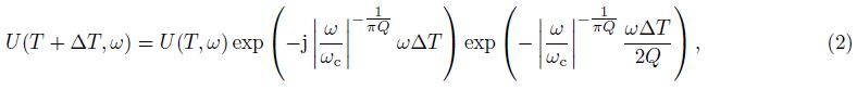
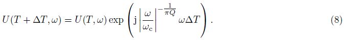
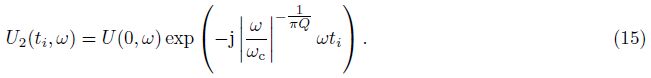
2 SEISMIC WAVE VISCOELASTIC ATTENUATION AND COMPENSATION 2.1 The Earth Q-FilterFutterman has proposed an equation to express the effect of amplitude attenuation and phase velocity dispersion for the earth Q-filter. The earth Q-filter can be based on the 1-D(two-way propagation)wave equation:

Eq.(1)has an analytic solution for one-way propagation, given by
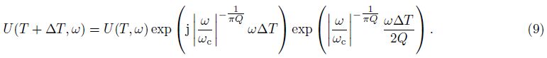
Then, we can have
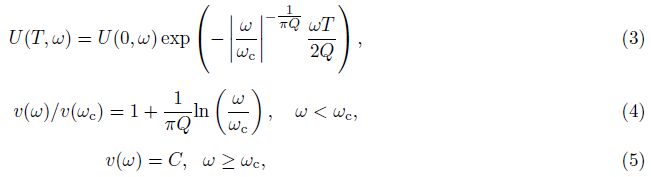
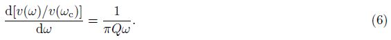
Based on Eq.(4), we can have
In Fig. 1, the trace of FFID=1 represents the synthetic trace using zero phase b and pass wavelet with central prequency 50Hz, and trace of FFID=2 represents the effect of earth Q-filter with constant Q=138 to the synthetic trace. We can see that seismic wavelet amplitude attenuates, dominant frequency decreases with time increasing, and then seiscmic wavelet is changed from zero phase to mixed phase.

|
Fig.1 The result of synthetic trace before and after inverse Q-filter |
In actual seismic data processing, there are different options of inverse Q-filter for different purpose.
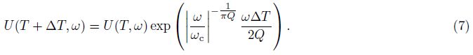
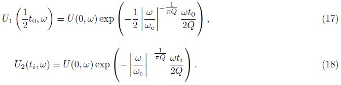
For only inverse Q-filter amplitude compensation, the expression of inverse Q-filter can be written as
For only inverse Q-filter phase compensation, there is
In Fig. 1, the trace of FFID=4 represents the result of inverse Q-filter phase compenastion, we can see that wavelet is restored to zero phase and phase dispersion is removed; trace of FFID=5 represents the result of inverse Q-filter amplitude and phase compenastion, then wavelet is fully restored to the zero phase b and pass wavelet with central prequency 50 Hz.
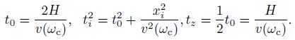
3 THEORETICAL ANALYSIS OF SEISMIC WAVE DISPERSION EFFECT 3.1 Theoretical ModelWe assume that the model is a homogeneous isotropic medium; H is the thickness of model; Q is medium quality factor; surface seismic and zero-offset VSP records have the same source wavelet; U(0, ω)is amplitude spectrum of source wavelet; !c is reference radian frequency and υ(ωc)is seismic wave phase velocity of reference frequency ωc; ti is surface seismic wave propagation time of reference frequency at offset xi; geophone of zerooffset VSP is located at downhole depth H and tz is down-going direct wave propagation time of reference radian frequency. Then, we have
Here, we use the model described above and quantitatively analyze velocity dispersion between surface seismic data and zero-offset VSP data based on the following four cases of inverse Q-filter.
(1)Without inverse Q-filter amplitude and phase compensation
The case without inverse Q-filter amplitude and phase compensation is equivalent to using Eq.(2)for seismic wave forward calculation. Then, the amplitude spectrum of down-going direct wave in zero-offset VSP data can be expressed as
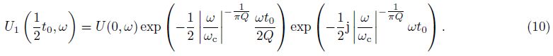
Amplitude spectrum of surface seismic wave at offset xi can be expressed as
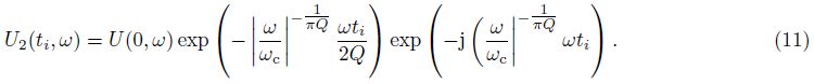
From Eqs.(10) and (11), we can see that amplitude attenuates, dominant frequency decreases, the relative energy of low-frequency increases with time increasing. When the propagation time of reference radian frequency tends to infinity, then seismic wave group velocity must be equal to the phase velocity of a specific frequency which is much smaller than the dominant frequency of source wavelet. According to Eq.(4), we can see that velocity dispersion increases and group velocity decreases with offset increasing. Here, we abbreviate seismic wave propagation time corresponding to group velocity as seismic wave propagation time.
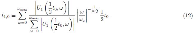
Thus, seismic wave propagation time is not only related to velocity dispersion, but also related to the relative energy of each frequency in seismic wave. Then, seismic wave propagation time can be expressed as the weighting of propagation time of each frequency component in seismic wavelet, and the weighting coefficient is the energy percentage of each frequency component in seismic wavelet amplitude spectrum. For zero-offset VSP data, seismic wave propagation time can be expressed as
For surface seismic wave at offset xi, seismic wave propagation time can be expressed as
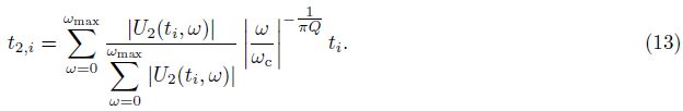
According to Eqs.(12) and (13), there is: t1, 0 < t2, i < t2, i+1. For surface seismic wave, the seismic wave propagation time is no longer hyperbolic. Therefore, after NMO and stacking to the reflection wave coming from depth H, time-depth relationship and waveform do not match the zero-offset VSP corridor stack data.
(2)Only inverse Q-filter amplitude compensation
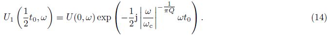
The case with inverse Q-filter amplitude compensation only is equivalent to using Eq.(2)for only considering velocity dispersion. Then, amplitude spectrum of down-going direct wave in zero-offset VSP data can be expressed as
Amplitude spectrum of surface seismic wave at offset xi can be expressed as
If only considering velocity dispersion, there is linear relationship between seismic wave propagation time and seismic wave propagation time of reference frequency. We assume that seismic wave propagation time of reference frequency is a unit time and seismic wave propagation time is α, then α > 1.
Thus, there are ${{t}_{1, 0}}=\frac{1}{2}\alpha {{t}_{0}}, {{t}_{2, i}}=\alpha {{t}_{i}}$, and
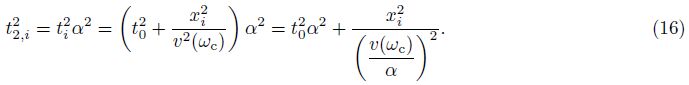
For surface seismic wave, although seismic wave propagation time is also hyperbolic, but when xi = 0, seismic wave propagation time is t0α. Therefore, after NMO and stacking to the reflection wave coming from depth H, time-depth relationship matches the zero-offset VSP corridor stack data, while waveform does not match.
(3)Only inverse Q-filter phase compensation
The case with inverse Q-filter phase compensation only is equivalent to using Eq.(2)for only considering amplitude attenuation. Then
There are ${{t}_{1, 0}}=\frac{1}{2}{{t}_{0}}$ and t2, i = ti. Then, phase spectrum of seismic wavelet at any time is same to the source wavelet.
For surface seismic wave, seismic wave propagation time is hyperbolic; and when xi = 0, seismic wave propagation time is t0. Therefore, after NMO and stacking to the reflection wave coming from depth H, the time-depth relationship and phase spectrum of seismic wavelet match the zero-offset VSP corridor stack data.
(4)Inverse Q-filter amplitude and phase compensation
The case of inverse Q-filter amplitude and phase compensation is equivalent to using acoustic wave equation for forward calculation. Amplitude spectrum of wavelet in surface seismic data and zero-offset VSP data is the same, and we can obtain

For surface seismic wave, seismic wave propagation time is hyperbolic; and when xi = 0, seismic wave propagation time is t0. Therefore, after NMO and stacking to the reflection wave coming from depth H, the time-depth relationship and waveform fully match the zero-offset VSP corridor stack data.
4 CASE STUDY OF VELOCITY DISPERSION AND INVERSE Q-FILTER PHASE COMPENSATION 4.1 Case Study of Velocity DispersionWe use zero-offset VSP data of dynamite and vibroseis source with same acquisition geometry as an example to verify the velocity dispersion expression derived in this paper.
For Z component of zero-offset VSP data, we pick the first break time firstly, and use it for wave field separation to obtain the down-going wave field, and then select seismic wave nearby the first break time as the down-going seismic wavelet. In seismic wavelet selection, we try to minimize the influence of multiple wave, and ensure that the amplitude spectrum of the selected seismic wavelet is as smooth as possible.
Figures 2a and 2b are amplitude spectrum of down-going seismic wavelet of dynamite and vibroseis source with the same acquisition geometry, respectively. In Fig. 2, the trace number increases with increasing depth of downhole geophone; colors represent energy. The acquisition geometry of dynamite and vibroseis source is the same, thus their travel paths are the same, functions of amplitude attenuation are the same, and also the functions of velocity dispersion.

|
Fig.2 (a) Spectrum of down-going wavelet with dynamite source; (b) Spectrum of down-going wavelet with vibroseis |
Comparing the amplitude spectrum in Figs. 2a and 2b at the same depth, we can see that when trace number changes from 26 to 236, the effective b and width of down-going wavelet for dynamite source is wider than that for vibroseis source; while trace number changes from 1 to 25, the effective b and width of down-going wavelet for dynamite source is narrower than that for vibroseis source. This is mainly caused by the source wavelet, as only a certain depth range of data can be recorded for each shot owing to the limits in the number of downhole geophones, and geophones are gradually lifted from the bottom to wellhead. Therefore, in order to obtain VSP records for whole depth of the well, several shots are needed. For dynamite source, the excitation environment is altered greatly after several times excitation, and then it causes lower dominant frequency and narrower b and width source wavelet. While for vibroseis source, the excitation environment is almost the same, then source wavelet is stable.
Figure 3a shows the first break time of down-going wavelet for dynamite source and vibroseis source, respectively; Figs. 3c and 3d show the difference and ratio of first break time, respectively. From Figs. 3c and 3d, we can see that the difference increases with depth increasing, but when trace number changes from 1 to 25, first break time for vibroseis source is less than that for dynamite source, as the difference is less than zero and ratio is less than 1.0. From Fig. 3d, we can see that the ratio increases with depth increasing, but the change rate decreases gradually.

|
Fig.3 The comparision of real first break time |
We can use amplitude spectrum of down-going wavelet for first break time inversion based on Eq.(12). We assume that ωc=300 Hz is reference frequency, fbi is seismic wave first break time of reference frequency at depth Hi, ${{\upsilon }_{i}}=1.062\frac{{{H}_{i}}}{f{{b}_{i}}}$ is seismic wave velocity of reference frequency and the unit is km/s, Qi = υi3 is average Q value between source and downhole geophone.
Figures 4a and 4b show the inverted seismic wave first break time of down-going wavelet for dynamite source and vibroseis source, respectively. Figs. 4c and 4d show the difference and ratio of the inverted first break time, respectively. When trace number changes from 1 to 25, the inverted first break time for vibroseis source is less than that for dynamite source, as the difference is less than zero and ratio is less than 1.0; and when trace number changes from 26 to 236, the inverted first break time for vibroseis source is greater than that for dynamite source, as the difference is greater than zero and ratio is greater than 1.0. The difference and ratio increases with depth increasing, which is consistent with the actual result(Fig. 3). But, affected by the accuracy of average Q value, reference frequency and phase velocity of reference frequency, only the trend of the inverted first break time matches the actual result. However, it still shows that velocity dispersion is not only related to propagation path and time, but also related to the relative energy of different frequency in seismic wavelet, and then it verified Eqs.(12) and (13).

|
Fig.4 The comparision of inverted first break time |
For another zero-offset VSP data, after first break time picking, wave field separation, NMO and corridor stacking, we obtain the corridor stack section of zero-offset VSP. Fig. 5 shows the calibration of zero offset VSP corridor stack section and surface seismic migration section, in order to calibrate the result of surface seismic data processing. In Fig. 5, trace numbers of 1-51 and 68-118 represent the surface seismic data nearby the borehole, while trace numbers of 55-64 represent the zero-offset VSP corridor stack section(one trace repeated ten times); trace numbers of 52-54 and 65-67 are filled with zero value. We can see that the surface seismic migration section and zero-offset VSP corridor stack section match with each other, but in some parts the surface seismic migration section does not match the zero-offset VSP corridor stack section.

|
Fig.5 The calibration of VSP corridor stack and surface seismic data nearby the borehole |
We can use amplitude spectrum of down-going wavelet for interval Q value inversion, and then use it for inverse Q-filter phase compensation to zero-offset VSP data and surface seismic migration data, the result is shown in Fig. 6. Compare Fig. 5 with Fig. 6, we can see that the match relationship is greatly improved after inverse Q-filter phase compensation.

|
Fig.6 The result after inverse Q-filter phase compensation |
We can calculate the cross-correlation coefficient of surface seismic migration data and zero-offset VSP corridor stack data before and after the inverse Q-filter phase compensation, in order to clearly analyze the effect of inverse Q-filter phase compensation. Fig. 7a shows the cross-correlation coefficient before inverse Q-filter phase compensation, Fig. 7b shows the cross-correlation coefficient after inverse Q-filter phase compensation and Fig. 7c shows the ratio of cross-correlation coefficient. For convenient display, trace numbers of 52-54 and 65- 67 are filled with 1.0. We can see that cross-correlation coefficient is improved after inverse Q-filter phase compensation, as the ratio is greater than 1.0(Fig. 7c).

|
Fig.7 The cross-correlation coefficient before and after inverse Q-filter phase compensation |
Based on Figs. 5-7, we can see that after inverse Q-filter phase compensation, the match of surface seismic data to VSP corridor stack data is effectively improved.
5 CONCLUSIONS AND SUGGESTIONSThe relationship of velocity dispersion between surface seismic data and zero-offset VSP data expressed in this paper can be used for seismic wave group velocity study.
In actual data processing, we should first apply inverse Q-filter phase compensation to surface seismic data and VSP data, so as to eliminate the effect of velocity dispersion and effectively increase the match of surface seismic data to VSP data, ultimately improve the credibility of seismic data.
6 ACKNOWLEDGMENTSThis work is supported by the National Nature Science Foundation of China(41174114).
| [1] | Badri M, Mooney H. 1987. Q measurements from compressional seismic waves in unconsolidated sediments. Geophysics, 52(6):772-784. |
| [2] | Bano M. 1996. Q-phase compensation of seismic records in the frequency domain. Bulletin of the Seismological Society of America, 86(4):1179-1186. |
| [3] | Bickel S H, Natarajan R R. 1985. Plane-wave Q deconvolution. Geophysics, 50 (9):1426-1439. |
| [4] | Blias E. 2012. Accurate interval Q-factor estimation from VSP data. Geophysics, 77(3):149-156. |
| [5] | Chen Z B, Chen X H, Li J Y, et al. 2014. A band-limited and robust inverse Q filtering algorithm. OGP (in Chinese), 49(1):68-75. |
| [6] | Futterman W I. 1962. Dispersive body waves. Journal of Geophysical Research, 67(11):5279-5291. |
| [7] | Gao J H, Yang S L. 2007. On the method of quality factors estimation from zero-offset VSP data. Chinese J. Geophys.(in Chinese), 50(4):1198-1209. |
| [8] | Gao J H, Yang S L, Wang D X. 2008. Quality factor using instantaneous frequency at envelope peak of direct waves of VSP data. Chinese J. Geophys. (in Chinese), 51(3):853-861. |
| [9] | Hamilton E L. 1972. Compressional-wave attenuation in marine sediments. Geophysics, 37(4):620-646. |
| [10] | Hargreaves N D, Calvert A J. 1991. Inverse Q filtering by Fourier transform. Geophysics, 56(4):519-527. |
| [11] | Hauge P S. 1981. Measurements of attenuation from vertical seismic profiles. Geophysics, 46(11):1548-1558. |
| [12] | Kjartansson E. 1979. Constant Q wave propagation and attenuation. Journal of Geophysical Research, 84(B9):4737-4748. |
| [13] | Liu C, Feng X, Zhang J. 2013. A stable inverse Q filtering using the iterative filtering method. OGP, 48(6):890-895. |
| [14] | Sams S M, Neept J P, Worthington M H, et al. 1997. The measurement of velocity dispersion and frequency-dependent intrinsic attenuation in sedimentary rocks. Geophysics, 62(5):1456-1464. |
| [15] | Spencer T W, Sonnadt J R, Butlers T M. 1982. Seismic Q-stratigraphy or dissipation. Geophysics, 47(1):16-24. |
| [16] | Stainsby S D, Worthington M H. 1985. Q estimation from vertical seismic profile data and anomalous variations in the central North Sea. Geophysics, 50(4):615-626. |
| [17] | Toksoz M N, Johnston D H, Timur A. 1979. Attenuation of seismic waves in dry and saturated rocks:1. Laboratory measurements. Geophysics, 44(4):681-690. |
| [18] | Tonn R. 1991. The determination of the seismic quality factor Q from VSP data:A comparison of different computational methods. Geophysical Prospecting, 39(1):1-27. |
| [19] | Wang X J, Yin X Y. 2011. Estimation of layer quality factors based on zero-phase wavelet. Progress in Geophys. (in Chinese), 26(6):2090-2098. |
| [20] | Wang Y H. 2002. A stable and efficient approach of inverse Q filtering. Geophysics, 67(2):657-663. |
| [21] | Wang Y H. 2003. Quantifying the effectiveness of stabilized inverse Q-filtering. Geophysics, 68(1):337-345. |
| [22] | Wang Y H. 2006. Inverse Q-filter for seismic resolution enhancement. Geophysics, 71(3):51-60. |
| [23] | Xu C D, Stewart R R. 2006. Seismic attenuation (Q) estimation from VSP data. CSEG National Convention, Extended Abstracts, 268-277. |
| [24] | Yan H Y, Liu Y. 2009. Estimation of Q and inverse Q filtering for prestack reflected PP-and converted PS-waves. Applied Geophysics, 6(1):59-69. |
| [25] | Yao Z X, Gao X, Li W X. 2003. The forward Q method for compensating attenuation and frequency dispersion used in the seismic profile of depth domain. Chinese J. Geophys. (in Chinese), 46(2):229-230. |
| [26] | Zhao J, Gao J H, Wang D X, et al. 2013. Estimation of quality factor Q from pre-stack CMP records. Chinese J. Geophys.(in Chinese), 56(7):2413-2428. |