1 INTRODUCTION

Acoustic waves are an important energy transfer form in the atmosphere. Some of the special events are sound sources which radiate acoustic waves in nature, such as earthquakes(Mutschlecner and Whitaker, 2005), Tsunamis( Le Pichon et al., 2005), Aurora(Wilson et al., 2005), lightning(Assink et al., 2008) and volcanic eruptions(Garcé's et al., 1999). These radiated acoustic signals naturally contain the relevant information of radiators and can be received by acoustic monitoring network when they propagate in the atmosphere( Le Pichon et al., 2009). Analyzing these acoustic signals is important to monitor natural events and underst and target sound sources. It is the atmosphere that conects the target sound source and acoustic sensors. The study of physical processes of acoustic wave propagation in the atmosphere is important for us to locate sound sources, underst and the evolution and deformation of acoustic signals(Drob et al., 2003).

Propagation of acoustic waves can be affected by atmospheric conditions. Generally, the atmospheric wind field and temperature gradient can refract acoustic wave propagation paths, and atmospheric density gradient makes the amplitude of the uplink acoustic wave power exponential growth, while the presence of dissipation in the atmosphere causes energy attenuation of acoustic waves. In the calculation of the acoustic wave propagation over a long distance, such as stratospheric ducting and thermospheric ducting with a propagation distance of more than 100 km(Drob et al., 2003), the dissipation effect on propagation trajectory of acoustic waves is often neglected. For example, acoustic wave propagation ray tracing in the atmosphere has been calculated under the wind field and temperature gradient background in the classical atmospheric acoustic ray model HARPA(Jones et al., 1986), WASP(Dessa et al., 2005) and (Tau-PGarcs et al.), ignoring attenuation effect. In these three ray models, the attenuation coefficient is introduced only to calculate the path loss by integrating the acoustic attenuation over ray path in the propagation process. In classical ray theory, the attenuation is only considered in the energy loss calculation, and the impact on ray trajectory has not been considered. Song et al.(2011)proposed acoustic ray tracing in the dissipative atmosphere on the basis of theoretical studies of lossy acoustic ray tracing. The calculation results show that the atmospheric dissipation has an impact on ray propagation trajectory of acoustic waves, but the physical mechanism of the dissipation effect on acoustic wave propagation trajectory is not well explained. The sound wave propagation process in a dissipative medium is simulated by using the FDTD method to study the impact of dissipation effect on acoustic wave propagation in this paper.

The finite-difference time-domain simulation which gives full-wave solution is an important method to study physical mechanism of acoustic wave propagation. Increasing studies of the acoustic propagation in the dissipative atmosphere have been made by using FDTD simulation. For instance, Wochner et al.(2005)established a numerical model of the finite amplitude acoustic in the real-dissipative atmosphere to simulate the evolution of each harmonic and wave energy attenuation in one dimension case by applying dispersion relation preserving. de Groot-Hedlin(2008)established a linear acoustic propagation model in the dissipative atmosphere to simulate amplitude changes of the wave packet propagating in the constant absorption atmosphere, and gave the channel attenuation characteristic of horizontal propagation in the dissipative atmosphere. Previous numerical studies of wave propagation in the dissipative atmosphere are mainly confined to the one-dimensional simulation, and mostly concern about the effect of dissipation on energy attenuation, lacking of attention on wave propagation trajectory in the dissipative atmosphere.

By using dispersion relation preserving difference scheme in space and third-order Runge-Kutta scheme with TVD property in time, a finite-difference time-domain model of acoustic wave propagation in a dissipative atmosphere is established in this paper. By simulating the monofrequency Gaussian acoustic wave packet propagate on different dissipation profiles and propagation under the same dissipation but at different frequencies, the influence of atmospheric dissipation on the wave trajectory and amplitude is studied from the point view of energy.

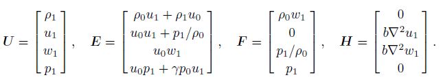
2 GOVERNING EQUATIONS

In the dissipative atmosphere, the dynamics equations describing atmospheric motion(Beer, 1974)can be expressed as follows:

where $\frac{d}{{dt}}$=α_t+V· ▽.(1)is the Navier-Stokes equation;(2)is the continuity equation, and (3)is the state equation describing the adiabatic process. p, ρ and V represent the atmospheric pressure, density and velocity, respectively; ξ and η denote the shear and bulk viscosity; γ=$\frac{{{c_P}}}{{{c_V}}}$ is specific heat ratio(c_p=1005 J·kg^-1·K^-1 is the specific heat at constant pressure and c_v=718 J·kg-1·K-1 is specific heat at constant volume); g is the gravitational acceleration.

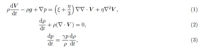
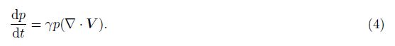
Combined the Eqs.(2) and (3), the Eq.(3)becomes:

Simplifying equations under the assumption of horizontal stratification, ignoring the atmospheric convective motion in the vertical direction, the pressure p, density ρ and fluid velocity V =(u, w)are decomposed into the background value(using the subscript 0) and acoustic disturbances value(using the subscript 1), separately:

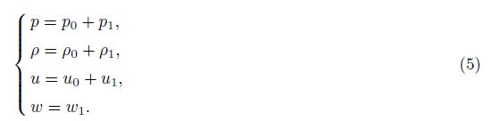
As the research target is usual irrotational acoustic waves, hence ▽▽·V ₁ = ▽²V₁. Under high-frequency approximation of acoustic waves, ignoring the gravity term in(1), linearizing the equations, the governing equation of wave propagation can be written as

where The inhomogeneous term H is composed of dissipation terms; where b =$\left({\xi + \frac{4}{3}\eta } \right)$/ρ₀ is the kinematic viscosity coefficient. This coefficient will be defined and modified as a dissipation coefficient to characterize the dissipation in this article.

3 NUMERICAL METHOD 3.1 Difference Equation

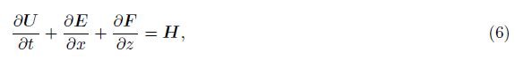
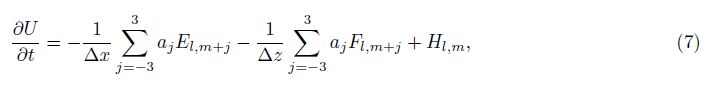
In general, the propagation scope of acoustic wave is vast in the atmosphere, so the space scale of numerical calculation is much larger than the acoustic wavelength. In a large-scale calculation grid, the amplitude difference of the acoustic wave source and acoustic waves in a far field is also great. This special simulation case requires a numerical method of higher accuracy. The dispersion relation preserving space difference scheme which has been widely used in aeroacoustics(Tam and Webb, 1993)is applied to spatial difference of governing equation, and the Runge-Kutta scheme is used to solve differences in the time domain. This difference scheme is of high accuracy, weak numerical dissipation and numerical dispersion.

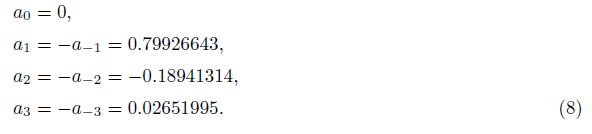
First, applying 7-point central difference dispersion relation preserving for governing Eq.(6), yields

where △_x and △_z are the horizontal and vertical space step, respectively. Tam and Webb(1993)have given a set of weight coefficients for the 7-point dispersion relation preserving difference scheme

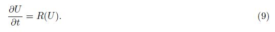
As the acoustic wave propagation is a fast, adiabatic process, besides the computational grid is large, the explicit time format of numerical simulation is adopted. In order to have a good calculation stability, a third-order time precision Runge-Kutta method with TVD properties developed by Shu and Osher(1988)is used.

Eq.(7)can be simplified into

The third-order Runge-Kutta method is expressed as: where △t is the time step; the old time step is denoted by the superscript n, and the new time step is denoted by the superscript(n + 1); U^k(k = 0, 1, 2, 3)are intermediate variables in the calculation.

3.2 Artificial Viscosity

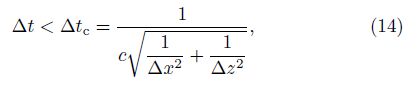
In numerical calculation with the central difference scheme, grid oscillation is a kind of common numerical noise. In order to ensure the accuracy of numerical simulation, artificial viscosity is applied to eliminate this noise. The artificial viscosity term is generally written as

where ν_a is artificial viscosity. Performing Fourier transform on Eq.(11), the attenuation term in the right-h and of Eq.(11)can be expressed as

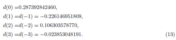
Tam(1995)presents a set of difference coefficients of the artificial viscosity term for 7-point difference scheme

The relationship between artificial viscosity coefficient D(α△x) and α△x for the 7-point difference scheme is shown in Fig. 1. It is seen that the attenuation effect of artificial viscosity on the acoustic fluctuation is almost zero when the value of α△x is less than 1. The artificial viscosity of 7-point difference scheme shows characteristics of blocking high frequency and passing low frequency. In numerical simulation, the oscillatory waves are well inhibited, while the simulated acoustic object is preserved.

3.3 Time Step and Boundary Conditions

For an explicit time scheme, the time step should satisfy the Courant stable condition in numerical simulation

where c is the adiabatic acoustic velocity. Since a smaller time step can improve the calculation accuracy, we set △t = 0.45△t_c.

The effects of different dissipation backgrounds on acoustic Gaussian wave packet propagation in an unbounded space are studied in this paper. Boundary reflection makes fluctuation interference in space, leading to accumulation of energy, interfering with the effect of acoustic wave propagation in the unbounded space. So an outflow boundary(Bogey and Bailly, 2002)is applied as a non-reflecting absorbing boundary condition in the simulation.

4 EXAMPLES

The influence of dissipation on acoustic wave propagation is mainly studied in this paper, so the numerical simulations here are in different profiles of dissipation coefficients, while atmospheric background density, temperature and pressure are constant. Thus, the impact of inhomogeneous density, temperature, and pressure on acoustic wave propagation can be avoided in the comparison of numerical simulation results while the dissipation effects can be clear. Hence, the dissipative effect can be quantitatively studied by constructing different profiles of dissipation coefficients. Propagation of sound waves at different frequencies are also simulated and analyzed for the same dissipation coefficient profile.

4.1 Single-frequency Acoustic Wave Propagation in Different Backgrounds

Firstly, single frequency acoustic wave packet propagation in different dissipative backgrounds is studied, including:(1)zero absorption(b = 0), i.e., an ideal case without dissipation;(2)absorption varies with height (b ≠ 0, $\frac{{{\rm{d}}b}}{{{\rm{d}}z}}$ ≠ 0); and (3)dissipation coefficient is constant(b ≠ 0, $\frac{{{\rm{d}}b}}{{{\rm{d}}z}}$= 0), i.e., a constant absorption case. A 50 Hz Gaussian sound wave packet is emitted in the horizontal direction, propagating through the constructed background medium. The mathematical form of Gaussian sound wave pressure packet is

where p_c and (x_c, z_c)are the amplitude of the sound pressure and center position of the acoustic wave packet, respectively; σ_x and σ_z are half wave width in the horizontal direction and vertical direction, respectively; and k_x and k_z are the horizontal and vertical component of the acoustic wave packet wave number, respectively. The frequency is set to 50 Hz, and acoustic wave packet horizontal emission with the elevation of 0° in the simulation, thus k_x = 0.924, k_z = 0. In order to accurately characterize the propagation of acoustic waves, we take △_x = △_z = λ/16, acoustic wavelength λ = 6.8 m, i.e. in the horizontal direction or the vertical direction, there are 16 mesh points on an acoustic wavelength scale.

Set the wave packet center x_c=42.92 m, z_c=212.9 m. σ_x and σ_z are control parameters of wave packet geometric spreading effect. Since this work focuses on the effect of background attenuation on acoustic waves, the geometric spreading effect should not be too strong, then, we take σ_x=53.125 m, σ_z=10.625 m.

4.1.1 Zero absorption case

In the background shown in Fig. 2A, the sound speed profile is a constant value, and the acoustic attenuation coefficient is 0. According to the classical scattering theory, acoustic wave propagation trajectory is a straight line in the ideal uniform zero absorption atmosphere, and the attenuation of acoustic wave is only caused by the geometric spreading in the space. The theoretical description of acoustic behaviors is consistent with the simulation results in Fig. 2B.

The propagation process is recorded in Fig. 2B. The horizontal coordinate of acoustic wave packet changes at the times 1.5 s, 3 s and 4.5 s, which means that acoustic waves take a corresponding displacement within 1.5 s. Comparing the vertical coordinate of the packet of the four moments, positions of the packet do not change significantly, which indicates that the acoustic wave packet propagates horizontally along the straight line. Comparing the moments 4.5 s and 0 s, the sound wave packet shows the longitudinal extension perpendicular to the propagation direction after spreading a certain distance, while sound pressure attenuates when comparing the sound pressure amplitudes of two moments. The effects of waveform extension and amplitude attenuation are caused by the geometric diffusion.

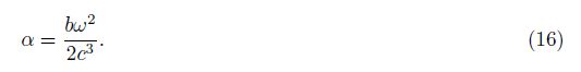
4.1.2 Varied absorption case

The profile that dissipation coefficient varies with height is structured as follows, suppose that dissipation coefficient is b = 0.01z m²/s. According to the sound attenuation theory, acoustic attenuation coefficient α can be expressed as

The profiles of sound velocity and attenuation coefficient are given in Fig. 3A. According to the classical ray theory, acoustic wave propagation trajectory is determined by the profiles of adiabatic sound velocity and wind speed. Based on the background in Fig. 3A, temperature is constant and there is no influence of wind field, thus sound wave propagation should be horizontal transmission. However, the simulation results show different phenomena from the classical ray theory in Fig. 3B.

Similar to Fig. 2B, the wave displacement of the packet generated in horizontal direction and the waveform extension caused by geometric spreading can be seen from the vertical and horizontal axes of Fig. 3B. In a dissipative medium, the acoustic energy attenuation is not only caused by geometric diffusion, but also by medium absorption. Comparing Fig. 3B with Fig. 2B, sound pressure of the packet in the former is significantly weaker than in the latter for the corresponding moments 1.5 s, 3 s and 4.5 s. However, the large sound pressure amplitude portion of packet gradually declines with propagation time(Fig. 3B)compared with Fig. 2B, while acoustic wave packet in Fig. 3B exhibits different waveforms from Fig. 2B. At 0 s moment, the symcenter of the wave packet is at the height of 212.9 m. After 4.5 s, the sound pressure center has a significant downward shift to the height between 150~200 m. As the attenuation coefficient of the background medium increases with height, attenuation coefficient in the upper part of the wave packet is larger than the lower part, and energy attenuation in the upper part is more than the lower part during the wave propagation, and sound pressure amplitude of the lower part of wave packet is gradually stronger than the upper part, resulting in the shifting of the package energy center.

4.1.3 Constant absorption case

The constant absorption background is shown in Fig. 4A, and the dissipation coefficient of wave packet center is set to b = 2.125 m²/s at the initial moment when the dissipation coefficient changes with height. Applying acoustic attenuation coefficient calculation formula(16), the profile of acoustic attenuation coefficient is given in Fig. 4A.

Obviously, waveform of the packet in Fig. 4B is almost the same as that in Fig. 2B at each time, and the waveform extension caused by the geometric spreading can be observed with the symcenter of the packets almost at the same horizon line. Different from Fig. 2B, the sound pressure intensity of the packet in the constant absorption case is weaker than the zero absorption case at 1.5 s, 3 s and 4.5 s moments due to the background atmospheric dissipation. The phenomena in Fig. 4B are in line with our underst and ing of propagation attenuation based on the classical ray theory. Meanwhile, it indicates that all parts of the wave packet energy simultaneously attenuate and wave packet center will not move during propagation in the constant absorption case.

4.2 Wave Energy Analysis for Three Cases

For zero absorption, varying absorption and constant cases, the simulation results of the packet waveform evolution in each case have been shown in Fig. 2 to Fig. 4. The waveform of the packet represents the wave energy distribution in space, and the intension and trajectory of acoustic energy are also of great importance to atmospheric acoustic wave propagation. The acoustic energy density can be expressed as

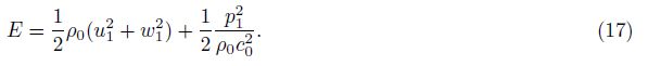
Sound fields are calculated by applying Eq.(17)for the three cases, obtaining the distribution of acoustic energy in space, where the energy center of the package is the position of maximum acoustic energy in the distribution. The energy propagation trajectories of packet can be obtained by presenting the energy center in space, as shown in Fig. 5a.

As shown in Fig. 5a, in the cases of zero absorption and constant absorption(data represented by "+" and "□", respectively), the trajectories of sound wave energy centers almost coincide and emerge horizontal transmission, which is consistent with the description of atmospheric acoustic ray theory. But for the varying absorption case(data represented by "△"), energy centers of the wave packet are gradual downward with propagation distance increasing. The trajectories of the packet represented by "△" that dissipative varies with height is different from classical ray theory, which indicates that classical ray theory without consideration of dissipation has some limitations. When the wave packet propagates in the varying absorption background, inhomogeneous dissipation coefficient will produce different effects on different parts of the wave package. The slope of dissipation coefficient in this case is $\frac{{{\rm{d}}b}}{{{\rm{d}}z}}$> 0, where the upper part of background dissipation coefficient is greater than the lower part, and the attenuation of the upper part of wave packet is greater than the lower part after propagation same distances, resulting in shifting of energy centers. Suppose the slope of dissipation coefficient profile is $\frac{{{\rm{d}}b}}{{{\rm{d}}z}}$< 0, i.e., dissipation coefficient decreases with height increase, then the attenuation of the lower part of wave packet is greater than the upper part, and the energy center will shift upward. This indicates that the inhomogeneous dissipation coefficient will deflect propagation trajectory, and the energy centers of the package shift to the area where attenuation coefficient is weaker.

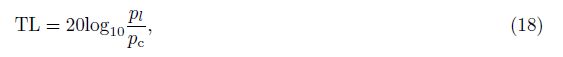
The transmission loss evolution of the acoustic energy center with distance is given in Fig. 5b for the three cases, where the transmission loss is defined as

where p_l is the sound pressure amplitude at the energy center of the packet shown in Fig. 5a; and p_c is the sound pressure amplitude of acoustic energy center at the initial time.

In Fig. 5b, the transmission loss of zero absorption case(represented by "□")is minimum, and that of the constant absorption case is maximum(denoted by "+"), while the transmission loss of the varies absorption case(represented by "△")is between the two cases after the acoustic wave packet propagating about 1400 m. This indicates that varies absorption not only changes the wave propagation trajectory deflecting to the weaker dissipation areas, but also reduces the acoustic energy loss compared with the constant absorption case. We use radiation transmission theory to analyze this energy loss mechanism, and the analysis results are shown in Fig. 6.

According to the ray theory, the transmission loss TL of the sound pressure center of acoustic wave packet can be decomposed into the attenuation L_G caused by geometric spreading of the acoustic wave packet and attenuation L_A caused by atmospheric sound absorption, i.e.

where units of L_G and L_A are dB. The atmospheric acoustic absorption can also be thought as the transmission loss along wave propagation trajectory. L_A can be theoretically expressed as where l is ray path, and α is the attenuation coefficient of the ray path in Eq.(20).

The profiles of attenuation coefficients for the three cases has been shown in Figs. 2A, 3A and 4A, and the wave propagation trajectories are given in Fig. 5a, respectively. According to Eq.(20), atmospheric sound absorption of the three cases can be calculated, and the results are shown in Fig. 6a.

In Fig. 6a, comparing the data represents by "△" and "+", inhomogeneous dissipation effects of the packet are not obvious as the wave propagation time is short and propagation distance is small at the initial time for the varying absorption case, while "△" and "+" roughly coincide. But with the increase of wave propagation distance, the sound absorption represented by "△" is gradually less than "+". The energy centers of the wave packet gradually move down due to the impact of inhomogeneous dissipation, and attenuation coefficient downward is less than the initial moment. Thus, the sound absorption of the wave packet energy center in the varying absorption case is less than the constant absorption case.

According to the transmission loss TL and atmospheric sound absorption L_A, the geometric spreading L_G can be obtained from Eq.(19)for the three cases(Fig. 6b). As shown in Fig. 6b, geometric spreading attenuation of the wave packet in the zero absorption case is the largest, while is smaller in the absorption case which is represented by "△" and "+". This also means that the shape of the packet has been greatly extended in the zero absorption case, the extension of packet shape is inhibited in absorption case. Contrasting the data indicated by "△" and "+", we find that the geometric spreading attenuation in the varying absorption case is greater than the constant absorption case after propagating 1400 m. This perhaps is because the trajectory length of the packet energy center in the varying absorption case is longer than the constant absorption case. Trajectory represented by "△" and "+" constitutes a right-angle side and hypotenuse in Fig. 5a, and the hypotenuse represented by "△" is clearly greater than the length of right-angle side represented by "+". Since the strength of geometric spreading attenuation depends on the extension degree of waveform, extension of waveforms is related to the propagation distance. A longer propagation distance results in a relatively greater waveform extension and causes a corresponding increase in geometric spreading.

Combining Fig. 6a with Fig. 6b, we can see that atmospheric sound absorption of the packet energy center in the varying absorption case is significantly less than the constant absorption case due to the impact of the path deflection; while compared with the zero absorption case, geometric spreading of the packet energy center also has some reduction.

4.3 The Acoustic Behaviors of Different Frequencies in Varies Absorption Case

For a given dissipation coefficient b, attenuation strength of acoustic wave of different frequencies are different as the attenuation strength depends on frequency, so we simulate the propagation of acoustic wave packet with the same scale and different frequencies in the varying absorption case to study the impact of the inhomogeneous dissipation on sound waves at different frequencies. Based on the parameters in Section 4.1.2, the frequency is 50 Hz in the case absorption varying with height; the background, the position of wave packet center and half-width parameters are not changed, while acoustic frequencies are set to 40 Hz and 60 Hz, respectively. Here we still are from the viewpoint of energy to analysis the position changes and energy loss of wave packet energy center in the dissemination process.

Propagation trajectories of the packet energy center of three frequencies are studied first. As shown in Fig. 7b, trajectory of energy center of 50 Hz wave packet is between the trajectories of 40 Hz and 60 Hz. After spreading about 1400 m, locations of the packet energy center at 40 Hz, 50 Hz and 60 Hz are offset by 28.5 m, 38.6 m and 56.9 m compared with the initial time, respectively. These results are similar to the Newton's prism experiment. The propagation trajectories of sound wave of different frequencies in the same varying absorption background are not same, which is a typical dispersion. This indicates that sound waves at different frequencies can generate dispersion in the inhomogeneous dissipation background during the propagation process. Comparing offset relationship of the three frequencies, we can see that the higher the acoustic wave frequency, the larger the offset of acoustic energy center in the case absorption varying with height. This phenomenon is related to the profile of acoustic attenuation coefficients.

According to Eq.(16), acoustic attenuation coefficient is proportional to the square of acoustic frequency, and attenuation coefficient profiles of the three frequencies under this dissipation coefficient background are shown in Fig. 7a, where the slopes of different sound attenuation coefficients are different in the same dissipation coefficient profile, the slope order according to descending order is 60 Hz, 50 Hz and 40 Hz. Combining Fig. 3 in Section 4.1.2, as the acoustic attenuation coefficient varies with space, the slope of the attenuation coefficient is not zero, and the attenuation of upper and lower part of wave packet is different, resulting in a shift of the wave packet energy center in the propagation process. Obviously, the greater the slope of acoustic attenuation coefficient, the greater difference the attenuation of upper and lower part of wave packet, the stronger the offset trend of energy center, and the energy center offset is the maximum after spreading a certain distance.

Transmission loss versus the propagation distance of the packet energy center of three frequencies is given in Fig. 7c where the trend is similar to Fig. 7b, and the higher the frequency, the greater the transmission loss. This phenomenon is consistent with our underst and ing of the classical wave propagation theory. This trend is determined by the acoustic wave attenuation and the propagation trajectory. As the acoustic frequency gets higher, the greater the attenuation coefficient is, and the trajectory length gets longer, as shown in Fig. 7b. Thus, the higher the frequency of the acoustic, the greater the transmission loss would be.

5 DISCUSSION

In the previous section, the acoustic wave packet of 0° transmission elevation in horizontal direction under the background absorption varying with height is simulated. The results indicate that the upper and lower parts of the packet attenuate at different levels, and the energy distribution of wave packet is changed, resulting in the energy center shifting to weaker dissipation areas. This mechanism is of great help for us to underst and acoustic wave propagation with nonzero elevation in the inhomogeneous dissipation background. The major axis of wave packet is parallel to the vertical direction when horizontally emitted. As for the packet with nonzero emission elevation, there is a certain angle between the vertical direction and the major axis. Since the absorption varying with height, different attenuation will present in different parts of the wave packet, and the bigger attenuation difference between the upper and lower part of the packet means larger height difference, which indicates that the bigger projection of major axis in the vertical direction. Thus, the projection of major axis of wave packet is the longest in the vertical direction, and the attenuation difference of the upper and lower part of wave packet is the biggest, and the deflection trend of wave propagation in the weak dissipation direction is the maximum when the acoustic is horizontally emitted. With the increase of launch elevation, the projection of the major axis gradually decreases in the vertical direction. Although the waves will deflect to weaker dissipative direction in the propagation, the offset of wave energy center is smaller compared with the horizontal emission case. When the launch elevation is 90°, there is no projection in the vertical direction, and the attenuation difference of the ends of wave packet disappear, so the energy center of the packet will not deflect to the weaker dissipative direction in acoustic propagation process. In order to validate acoustic wave packet under the background of zero absorption and varying absorption with elevation of 90°, the simulation results are shown Fig. 8. Figs. 8a and 8b are the comparison results of the propagation trajectory and SPL at the wave packet center, respectively, where "□" denotes the calculation result of the zero absorption case, and "+" represents result of the case absorption varying with height. The comparison results show that the dissipative profile only affects the amplitude of sound waves and have no impact on the propagation trajectory when the emission angle is 90°.

Applying the ray theory to analysis transmission loss of energy center of 50 Hz wave propagating under the three different backgrounds, the transmission loss is decomposed into the geometric spreading and the atmospheric sound absorption attenuation along the propagation path. Undoubtedly, Fig. 6a shows the trajectory deflection of the packet energy center due to the varying absorption, and the atmospheric sound absorption of the packet energy center is significantly reduced. There are some special phenomenon in geometric spreading calculated by the transmission loss TL and atmospheric sound absorption LA. As shown in Fig. 6b, geometric spreading loss represent by "+" and "△" increases with the growth of propagation distance at the initial time, but the growth trend is significantly smaller compared with the zero absorption case. Geometric spreading attenuation is no longer growing and shows a slight decreasing trend after spreading some distance. During the interval of 1000~1500 m, geometric spreading loss increases approximately 0.4 dB in the constant absorption case and increases about 0.1 dB in the varying absorption case. In general, the geometric spreading loss shift from large to small means the waveform gather to a certain degree. Despite that this small rise may be due to the error caused by numerical calculation, there is the possibility that varying absorption would produce an aggregation effect on acoustic waves. The influence of background absorption on acoustic wave propagation needs to be further studied.

6 CONCLUSIONS

The high frequency acoustic wave propagation equations in the atmosphere is numerically solved by using dispersion relation preserving difference scheme in space and Runge-Kutta display scheme in time. The sound propagation of the same Gaussian wave packet in different backgrounds and the same wave packet parameters with different frequencies in the same absorption background are simulated, and the numerical simulation results are compared and analyzed.

The propagation of acoustic horizontal emission in the horizontal stratified dissipative atmosphere shows that the varying absorption atmosphere does have some impacts on wave propagation trajectory and energy consumption. Different parts of the wave packet receive different dissipations due to the varying absorption. The attenuation differences lead to the energy center of the packet to shift to the weaker dissipation direction and the propagation trajectory is deflected. This is much different from the prediction of classical ray theory without dissipation, which indicates that there are some limitations and constraints in the application of classical ray theory without consideration of absorption effect.

The inhomogeneous dissipation not only changes the propagation trajectory of energy center of wave packet but also modifies the transmission loss. The influences are concluded as follows:(1)Atmospheric sound absorption representing the path loss significantly reduces compared with the constant absorption case.(2) Geometric spreading attenuation is significantly inhibited compared with the zero absorption case. Since the acoustic attenuation is in proportional to the square of frequency, atmospheric dissipation will bring dispersion properties into acoustic propagation. Under the same varying absorption background, energy trajectories of wave packet at different frequencies are different. As the frequency of acoustic wave packet gets higher, the offset of energy center would be larger.

7 ACKNOWLEDGMENTS

This work was supported by the National Natural Science Foundation of China(41327002).