 2014, Vol. 57


2. University of Chinese Academy of Sciences, Beijing 100049, China;
3. National Center for Space Weather, China Meteorological Administration, Beijing 100081, China
Lyman-Birge-Hopfield(LBH)bands dayglow emissions in the ionosphere, produced by the photoelectrons impact on the nitrogen molecules, are the most prominent molecular signals in the far ultraviolet(FUV)emission range. Imaging the LBH dayglow emissions from the space provides not only the density of molecular nitrogen and oxygen(Meier, 1991), but also the message of the ionospheric photoelectron flux(Oran and Strickland , 1978), and can be a powerful method to monitor the state of the upper atmosphere. Thus, LBH emissions have been used as the observational objectives of satellite equipments, such as DMSP/SSUSI(Paxton et al., 1992), TIMED/GUVI(Paxton et al., 1999), and IMAGE/WIC(Mende et al., 2000). In China, the Wide-field Auroral Imager(WAI)aiming at observing the aurora and LBH dayglow emissions in the range of 140~180 nm will be carried on satellite FY-3D, and this instrument will be used to monitor the auroral activity and the space weather of the ionosphere.
Accurate underst and ing of the physical generation process of the LBH emissions and the establishment of an appropriate model are very important in deriving valid geophysical parameters. McEwen et al.(1966)disscussed the intensity distribution of the LBH bandsystem, but only presented the initial theoretical formula. Conway(1992)studied the self-absorption effect of molecular nitrogen for the radiative transfer of the LBH emissions, and pointed out that the absorption effect of oxygen dominates the self-absorption effect of molecular nitrogen. Dashkevich et al.(1993) and Eastes et al.(2000)discussed the effect of the radiative cascade between the excitation states. On the basis of previous works, Strickland et al.(1995) and Evans et al.(1995)put forward the common theoretical model for the LBH dayglow emissions. Recently, computational models and associated computer codes for ultraviolet radiance and transmission are under active development(Huffman, 1992). However, only a few codes can be used for calculation of the FUV emissions besides AURIC(Atmospheric Ultraviolet Radiance Integrated Code), which is developed by the Computational Physics, Inc. and the Air Force Phillips Laboratory/Geophysics Directorate(Link et al., 1992; Strickland et al., 1992). In calculating LBH column emissions rates, AURIC treated the solar zenith angle(SZA)as a constant along the line of sight(LOS), and Strickland et al.(1999)pointed out that AURIC is restricted to SZAs less than 90°. So, AURIC is only useful for the instruments with small instantaneous field of view(FOV). For example, DMSP/SSUSI and TIMED/GUVI, whose instantaneous FOVs are both 11.8°. These two instruments were operated at the altitudes of 830 km and 630 km respectively. When their FOVs are both projected to the altitude of 155 km, the maximum difference of the SZAs in the FOV is 1.2°(details in Appendix A). However, for the large instantaneous FOV of the WAI(FOV=130°), the maximum difference of the SZAs in the FOV is 50° at the same altitude(details in Appendix A), and we must consider the effect of SZA and treat it as a variable along the LOS.
In order to meet the requirement of studying the LBH dayglow emissions for the large FOV, this paper presented a revised method(named as RAURIC)to calculate the column emission rates of the LBH dayglow emissions based on AURIC. RAURIC used the atmospheric model with spherical geometry, treated the SZA as a variable along a LOS, and improved the limitations of AURIC. The arrangement of the paper is as follows. The spectral synthesis for the LBH emissions and the method of calculating the LBH column emission rates will be first described in Section 2. Then, calculation results from both RAURIC and AURIC as well as discussions will be presented in Section 3. Finally, a brief summary will be given in Section 4.
2 LBH DAYGLOW EMISSIONS 2.1 Spectral SynthesisThe LBH bands are due to the transition

The bands are produced by the electric dipole forbidden transition from the excitation state(α1Πg)to the ground state(X1Σ g+). Between these two states, magnetic dipole and electric quadrupole transition are permitted according to the selection rules(Conway, 1992). Each LBH band consists of five branches(O, P, Q, R, S), three of which(P, Q, R)are a mixture of magnetic dipole and electric quadrupole corresponding to △J = -1, 0, 1, and the remaining two branches(O, S)are pure electric quadrupole corresponding to △J = -2, 2.
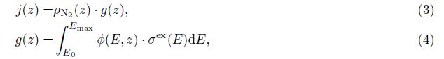
The volume emission rates of a LBH band is given by

As for the calculation of j(z), we adopt the direct excitation theory of electron impact, and it can be calculated by the product of g-factor g(z) and the density of molecular nitrogen ρN2(z)as follows:

|
Fig.1 Excitation cross sections of the α1Πg state |
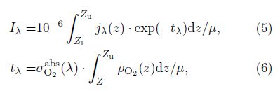
When the LBH dayglow emissions are imaged from space, the observed physical parameter is the column emission rate Iλ(in Rayleigh), which is calculated by integrating the volume emission rate and the probability of a photon traveling from a point to the observer without being scattered along a LOS

|
Fig.2 Observation geometry |
The calculation of the LBH volume emission rates has been discussed in Section 2.1, and the next step is to calculate the probability of a photon traveling from a point to the observer without being scattered. We consider the absorption effect of the oxygen and neglect the self-absorption effect of molecular nitrogen since the molecular nitrogen is optically thin to the LBH emissions(Conway, 1992). Therefore the scattering probability can be characterized by the optical depth of oxygen, and the absorption cross sections used in this work(Strickland et al., 1999)are shown in Fig. 3.

|
Fig.3 Absorption cross sections of molecular oxygen |
Figure 4 shows the steps of calculating the LBH column emission rates.

|
Fig.4 Flowchart of calculation of column emission rates |
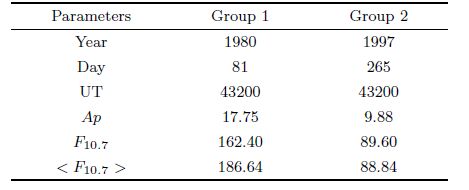
Step 1, Set up the input parameters. The input parameters which are used to specify the atmospheric model include date(Year, Day), time(UT), geomagnetic activity index(Ap), solar 10.7 cm flux(F10.7) and its 81-day averaged value(< F10.7 >). In order to study the LBH dayglow emissions at different levels of solar activity, we have chosen two cases("Group 1" for high activity and "Group 2" for low activity)as shown in Table 1.
| Table 1 Parameters of atmosphere model |
Step 2, Define the model boundaries. The ionospheric dayglow emissions are produced in the dayside upper atmosphere. The lower atmospheric region below 90 km has strong absorption effect on the LBH emissions, and the density of molecular nitrogen in the upper atmospheric region above 600 km is very low, so we set Zl = 90 km and Zu=600 km as the boundaries of the emission region. In this region, the atmospheric model is described by spherical geometry, i.e. the atmosphere is divided by a series of spherical layers. The interval between two layers is defined by the density structure of the upper atmosphere(Bush and Chakrabarti, 1995). Here, the emission region is divided into 43 layers(N=43), the same as AURIC.
Step 3, Define the LOS. First, the position of the detector(H, Φ, λ)should be given(i.e. altitude, latitude, and longitude). Secondly, the value of the observation angle should be given. However, the direction of the LOS has not been defined since the azimuth angle has not been given. Here, the azimuth angle β is defined by the angle from the east as the initial edge and then anti-clockwise to the LOS as the final edge.
Next step is to calculate the position of each column. The emission region has been divided into 43 layers, so there are 43 columns along the LOS. The altitude of each column is easy to define, but the latitude and longitude are difficult to calculate. Here, the technique of vertical projection is used to define the position of each column. Take the calculation of the top column for example. First, we vertically project a plane to the top column, and calculate the horizontal and vertical coordinates of the top column(x, y)in the plane. Then, we can use the formula of vertical projection(details in Appendix B)to transfer the horizontal and vertical coordinates(x, y)to the latitudinal and longitudinal coordinates(Glat, Glon). Other columns are calculated in the same way.
When the position of each column is defined, we can calculate the observation angle of each column. Accrooding to the definition of the observation angle, in a spherical atmosphere the nadir direction of each column changes along the LOS, so the observation angles of the 43 columns along the LOS are also different. As we have known the coordinates of the observer, we can know the vector of the LOS. Then, the vertical vector of each column can be easily calculated. Finally, the observation angle between the two vectors can be calculated.
Step 4, Call the atmospheric model MSISE-00 to calculate the density of each column. The coordinates of each column and the input parameters shown in Table 1 are used to drive the atmospheric model to derive the densities of molecular nitrogen ρN2(z) and oxygen ρO2(z).
Step 5, Calculate the volume emission rates of each column. Here, we use the module of volume emission rates in AURIC. In this step, we consider the variety of the SZA along the LOS, which is different from the algorithm of AURIC. AURIC treats the SZA as a constant along the LOS, and this treatment is completely appropriate in nadir, so for each column along the LOS direction we call the module of volume emission rates in AURIC once to calculate the volume emission rates in nadir with different SZAs. Once we have calculated the volume emission rates and given the data of fλ, we can calculate the volume emission rates of each LBH band jλ by Formula(2).
Here, we use the trapezoidal integration to define the values of each column(i.e. the values of each column equal to the average of the next column and the previous column), such as the density of molecular nitrogen ρN2(z), the density of the oxygen ρO2(z), the observation angle μ, and the volume emission rates jλ.
Step 6, Radiative transfer calculation. As for radiative transfer of the LBH emission, we just consider the absorption of the oxygen. Therefore we calculate the optical depth of each column along the LOS by Formula(6).
Finally, with these defined parameters of each column along the LOS, we can calculate the column emission rates of the LBH dayglow by Formula(5). The RAURIC mainly improves two limitations of AURIC, one is the definition of the observation azimuth angle and the other is treating the SZA as a variable along the LOS direction. These two improvements are very important to calculate the LBH dayglow emissions for large FOV, because the intensity of LBH emissions is strongly affected by the SZA(Huffman, 1992).
3 TESTS OF THE RAURICIn order to test the RAURIC, we calculated the LBH dayglow emission in the range of 140~180 nm. The results include the column emission rates in nadir and in other LOS’s. Then, we compare the results of RAURIC with those of AURIC.
3.1 Nadir ObservationThe column emission rates in nadir are shown in Fig. 5. The left and right columns are calculated by the two sets of atmospheric models presented in Table 1. In Fig. 5, the altitude of the observer is 830 km; the longitudes from the top to the bottom are 0°, 20°, 50°, respectively, and the range of the latitude is -80°~80°(in geographical coordinates). Fig. 5 clearly indicates that the results of RAURIC and AURIC are in agreement in nadir for both high and low activities.

|
Fig.5 Comparison of RAURIC and AURIC in nadir |
Figure 6 presents the results of column emission rates in other LOS’s. In Fig. 6, the altitude of the observer is 830 km, the coordinates from the top to the bottom are(20°, 20°), (35°, 35°), (50°, 50°), and the range of the observation angle is 0°~60°. We have used a spherical atmosphere in this work, so the azimuth angle should be given. We have chosen four azimuth angles 0°, 180°, 270°, 90°(i.e. East, West, South, and North).

|
Fig.6 Comparison of RAURIC and AURIC in other LOS |
Figure 6 shows that the calculation results of RAURIC and AURIC are in great agreement when the observation angle is less than 20°. However, as the observation angle increases, the difference of SZA increases, and the differences between the results of RAURIC and AURIC become clear. In Figs. 6a and 6b, the SZAs at East and North change more significantly than those at West and south, so the differences of RAURIC and AURIC also become more clear. In Figs. 6a and 6b, the differences become even clearer than those in Figs. 6a and 6b. With the further increase of the observation angle, the changes of SZA become more significant, and the differences between the results of RAURIC and AURIC become more apparent. Next, we will discuss the algorithmic difference between RAURIC and AURIC.
3.3 DiscussionsThe ionospheric LBH dayglow emissions are produced by the photoelectrons impact on the molecular nitrogen, and the intensity of LBH emissions has strong dependence on SZA(Huffman, 1992), so we should consider the variety of the SZA along the LOS. In order to show the dependence, we calculate the volume emission rates at four azimuth angles(i.e. East, West, South, and North). In Fig. 7, the altitude of the observer is 830 km, the latitude and the longitude are(50°, 50°), and the observation angle is 60°.

|
Fig.7 Comparison with volume emission rates of AURIC |
Figure 7 shows that the emission region which dominates the contributions to the LBH volume emission rates is between ~120 km and ~220 km. In this region, the volume emission rates of AURIC are obviously different from the results calculated by RAURIC.
Next, we discuss the relationship between g-factor and SZA. Here, we calculate the g-factors at the altitudes of 150 km and 180 km by Formula(4). In Fig. 8, the range of the SZA is 0°~90°, and the left panel and the right panel are calculated by the two atmospheric models of Table 1, respectively.

|
Fig.8 Relationship between g-factor and SZA |
Figure 8 shows that the g-factors at different altitudes have almost the same variety tendency. When the SZA is less than 40°, the variety of g-factor is small. However, when the SZA is greater than 40°, the variety of g-factor is very significant. Fig. 9 shows how the SZAs presented in Figs. 6e and 6f change with the view angles.

|
Fig.9 Relationship between view angle and SZA |
AURIC treats the SZA as a constant along the LOS, so the SZA does not change with the view angle. While RAURIC considers the SZA as a variable, so the SZA changes with the view angle. When the view angle is small, the SZA changes little. But when the view angle increases greatly, the SZA also changes greatly. Fig. 9 also shows that, when the view angle is 60° and the azimuth is East, the change of SZAs is 13° and the g-factor decreases about an order of magnitude. In a word, it is appropriate to treat the SZA as a constant for small FOV, while we should consider the SZA as a variable for large FOV.
In nadir, both AURIC and RAURIC treat the SZA as a constant along the LOS, so the column emission rates of AURIC and RAURIC are in good agreement as shown in Fig. 5. However, in other LOS’s, we should use RAURIC to calculate the LBH dayglow emissions, especially for large FOV.
4 CONCLUSIONIn this paper, we presented a spectral synthesis of the LBH dayglow emissions according to the direct excitation theory and the spherical geometry, and then proposed a revised method to calculate the column emission rates of the LBH dayglow emissions for large FOV. RAURIC considers the change of the SZA along the LOS. RAURIC improved the limitations of the module used to the volume emission rates in AURIC. Now, it is appropriate to use RAURIC for disk-viewing with SZAs less than 90°, but it is not applicable for limb-viewing with SZAs more than 90°.
RAURIC builds a solid basis for simulating the image of ionospheric LBH dayglow emissions and the data inversion technique. We will study the response of the LBH dayglow emissions to the ionosperic space weather(Ma et al., 2002; Xu, 2009) and develop the dayglow removal technique(Strickland et al., 1994; Gladstone, 1994)in the future work.
5 Appendix AIn Appendix Fig. 1, the radius of the Earth(R)is 6371.0 km, and the altitude of the observer(H)is 830 km.
|
|
Appendix Fig. 1 Geometrical sketch map |
(1)Difference of the SZAs for small FOV
Suppose the FOV angle(∠DAAE)to be 11.8°, which is the instantaneous FOV of both the DMSP/SSUSI and TIMED/GUVI, then the angle ∠OAE equals 5.9°. AD and AE intersect the circle at the altitude of 150 km, which is the typical projection altitude of the LBH dayglow emissions. OD is in the nadir direction of the point D, and OE is in the nadir direction of the point E. So the angle ∠DOE equals the difference of the SZAs between D and E.
According to the sine rule in △OAE
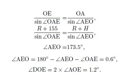
So, the difference of the SZAs between D and E is 1.2°.
(2)Difference of the SZAs for large FOV
When the FOV angle(∠CAB)is 130°, which is the instantaneous FOV of the Imager on FY-3, AB and AC are the tangents of the circle at the altitude of 150 km. CO is in the nadir direction of the point C, and BO is also in the nadir direction of the point B. So the angle ∠COB equals the difference of the SZAs between C and B.
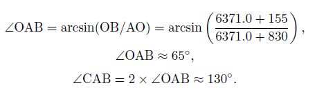
Because AB and AC are perpendicular to BO and CO respectively, the supplementary angle of ∠CAB is
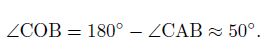
So, the difference of the SZAs between C and B is about 50°.
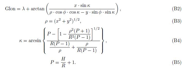
6 Appendix BVertical projection constructs the relationship between the geographical coordinates(Glat, Glon) and the horizontal and vertical coordinates(x, y). Then, we can transfer(x, y)to(Glat, Glon)by formula(Snyder, 1987)as follows: Glat = arcsin

This work is supported by the National Hi-Tech Research and Development Program of China(2012AA121-000), the National Basic Research Program of China(2012CB957800, 2011CB811400), the National Natural Science Foundation of China(10878004, 41274147, 41204102). We are grateful to Computational Physics Incorporation(CPI)for the AURIC code. And we thank the referees for their suggestions and assistance in evaluating this paper.
| [1] | Ajello J M, Shemansky D E. 1985. A reexamination of important N2 cross sections by electron impact with application to the dayglow:the Lyman-Birge-Hopfield band system and NI(119.99 nm). J. Geophys. Res., 99(A10):9845-9861, doi:10.1029/JA090iA10p09845. |
| [2] | Bush B C, Chakrabarti S. 1995. A radiative transfer model using spherical geometry and partial frequency redistribution.J. Geophys. Res., 100(A10):19627-19642, doi:10.1029/95JA01209. |
| [3] | Conway R R. 1992. Self-Absorption of the N2 Lyman-Birge-Hopfield bands in the far ultraviolet dayglow. J. Geophys.Res., 87(A2):859-866, doi:10.1029/JA087iA02p00859. |
| [4] | Dashkevich Z V, Sergienko T I, Ivanov V E. 1993. The Lyman-Birge-Hopfield bands in aurora. Planet. Space Sci., 41(1):81-87, doi:10.1016/0032-0633(93)90019-X. |
| [5] | Evans J S, Strickland D J, Paxton L J. 1995. Satellite remote sensing of thermospheric O/N2 and solar EUV, 2. Data analysis. J. Geophys. Res., 100(A7):12227-12233, doi:10.1029/95JA00573. |
| [6] | Eastes R W. 2000. Emissions from the N2 Lyman-Birge-Hopfield bands in the Earth's atmosphere. Phys. Chem. Earth, 25(5-6):523-527, doi:10.1016/S1464-1917(00)00069-6. |
| [7] | Gladstone G R. 1994. Simulations of DE 1 UV airglow images. J. Geophys. Res., 99(A6):11441-11448, doi:10.1029/93JA03525. |
| [8] | Huffman R E. 1992. Atmospheric Ultraviolet Remote Sensing. London:Academic Press. |
| [9] | Link R, Strickland D J, Daniell R E. 1992. AURIC airglow modules:phase 1 development and application. SPIE, Ultraviolet Technology IV, 1764:132-1441, doi:10.1117/12.140843. |
| [10] | Mcewen D J, Nicholls R W. 1966. Intensity distribution of the Lyman-Birge-Hopfield band system of N2. Nature, 209(5026):902, doi:10.1038/209902a0. |
| [11] | Meier R R. 1991. Ultraviolet spectroscopy and remote sensing of the upper atmosphere. Space Sci. Rev., 58(1):1-185, doi:10.1007/BF01206000. |
| [12] | Mende S B, Heetderks H, Frey H U, et al. 2000. Far ultraviolet imaging from the IMAGE spacecraft. 2. wideband FUV imaging. Space Sci. Rev., 91(1):271-285, doi:10.1023/A:1005227915363. |
| [13] | Ma S Y, Liu H X, Schlegel K. 2002. A comparative study of magnetic storm effects on the ionosphere in the polar cap and auroral Oval-F-Region negative storm. Chinese J. Geophys.(in Chinese), 45(2):160-169. |
| [14] | Oran E S, Strickland D J. 1978. Photoelectron Flux in the Earths Ionospheric. Planet. Space Sci., 26(1):81-87, doi:10.1016/0032-0633(78)90056-9. |
| [15] | Paxton L J, Meng C I, Fountain G H, et al. 1992. Special Sensor Ultraviolet Spectrographic Imager(SSUSI):An instrument description. SPIE, 1745:2-15, doi:10.1117/12.60595. |
| [16] | Paxton L J, Christensen A B, Humm D C, et al. 1999. Global ultraviolet imager(GUVI):measuring composition and energy inputs for the NASA Thermosphere Ionosphere Energetics and Dynamics(TIMED) mission. SPIE, 3756:265-276, doi:10.1117/12.366380. |
| [17] | Snyder J P. 1987. Map Projections-a Working Manual. Reston:U.S. Geological Survey. |
| [18] | Strickland D J, Evans J S, Bishop J, et al. 1992. Atmospheric ultraviolet radiance integrated code(AURIC):Current capabilities for rapidly modeling dayglow from the far UV to the near IR. SPIE, 2831:184-199, doi:10.1117/12.257195. |
| [19] | Strickland D J, Cox R J, Barnes R P, et al. 1994. Model for generating global images of emission from the thermosphere.Appl. Opt., 33(16):3578-3594, doi:10.1364/AO.33.003578. |
| [20] | Strickland D J, Evans J S, Paxton L J. 1995. Satellite remote sensing of thermospheric O/N2 and solar EUV, 1. Theory.J. Geophys. Res., 100(A7):12217-12226, doi:10.1029/95JA00574. |
| [21] | Strickland D J, Bishop J, Evans J S, et al. 1999. Atmospheric ultraviolet radiance integrated code(AURIC):Theory, software architecture, inputs, and selected results. J. Quant. Spectrosc. Radiat. Transfer, 62(6):689-742, doi:10.1016/S0022-4073(98)00098-3. |
| [22] | Xu W Y. 2009. Variations of the auroral electrojet belt during substorms. Chinese J. Geophys.(in Chinese), 52(3):607-615. |