1 INTRODUCTION

Pre-stack seismic imaging is a main method to explore the subsurface structure by extracting the information carried by seismic waves. With the development of exploration, structural imaging cannot meet the requirements and lithological imaging is needed. In other words, the true-amplitude imaging is necessary( Li ZC et al., 2008). Now, most of the true-amplitude imaging algorithms are based on the approximation of perfect elastic media, while the realistic subsurface is anelastic, especially near the surface and reservoirs. Seismic wave attenuation and dispersion caused by viscosity can lead to mislocated imaging points and under-estimated imaging amplitude if viscosity is not included in the imaging algorithm.

The conventional method to compensate the attenuation and dispersion caused by viscosity is the inverse- Q filter, which can improve the resolution by enhancing high-frequency components(Wang, 2002, 2006; Li Z C et al., 2007). This method is based on one-dimensional backward propagation and cannot correctly h and le real geological complexity(Zhang Y et al., 2010). Another method is inverse-Q migration, which is more accurate because attenuation and dispersion are corrected during wave propagation. There are mainly three inverse Q migration methods which are the methods based on the ray theory(Ribodetti et al., 1998), one-way and two-way wave equation. The method based on the ray theory is difficult to h and le multiple wavepaths, so the accuracy decreases in complex geology. The other two methods based on wave equation have higher accuracy. The main difficult in inverse Q migration is the instability encountered during the wavefield backward extrapolation. Mittet et al.(1995)firstly developed the strategies to compensate for attenuation and dispersion based on one-way wave equation migration, and then Zhang et al.(2002), Zhou LB et al.(2012)applied those strategies to different wave extrapolation operators. To stabilize the algorithm, frequency clipping of the gain function or the limited propagation direction was used. Besides the above methods, Wang et al.(2008)applied the stable factor method which was firstly used in the inverse Q filter to the invert Q migration(Wang et al., 2008). Zhang LB et al.(2010)combined the two methods to develop a more stable method. The instability problem is more serious in the two-way wave equation inverse Q migration. Causse et al.(1999, 2000)derived an amplifying medium and presented a stable backward propagation method by separating dispersion and amplitude terms. Although their method is stable, it is difficult to extend to other mechanical models. Recently, Deng et al.(2007, 2008)developed true-amplitude RTM in visco-acoustic and visco-elastic media, but they did not focus on the stable problem. Zhang Y et al.(2010)derived a new visco-acoustic wave equation from dispersion relationship and pointed out that the stability problem can be solved by adding a regularization term. Suh et al.(2012)extended the Zhang Y’s(2010)method to visco-anisotropic media and used a high-cut filter to make the algorithm stable. In a word, stability problem remains a main issue for the migration in viscosity media. Although some techniques can make the algorithm stable, some previous tests to choose suitable parameters are needed and the wavefield is damaged in most cases.

The history of least-squares migration(LSM)can be traced back to 1984, when Tanrantola gave the theory of linearized inversion of seismic data(Tanrantola 1984). Because of the heavy computation cost, this method was not be widely used until recently. The first attempt was the LSM based on Kirchhoff and one-way wave equation operator(Nemeth et al., 1999; Wang et al., 2009; Liu et al., 2013; Tang, 2009). In recent years, LSRTM based on the two-way wave equation was developed. Dai et al.(2012)developed 3D LSRTM and reduced the computation cost by introducing phase encoding technology. Yao et al.(2012a, 2012b)gave the theory and synthetical examples of linear and non-linear LSRTM. Dong et al.(2012)proved that LSRTM can preserve amplitude and has higher resolution by tests on synthetic and real data. Most of them were based on perfect elastic media, few took into account the viscosity of media. Based on the theory of LSM, Zhang CJ et al.(2010)obtained a time variant deconvolution operator which can be applied to the imaging result to correct attenuation. Mulder et al.(2009) and Hak et al.(2010, 2011)discussed the ambiguity of visco-acoustic LSRTM in frequency-space domain and applied those methods to linear and non-linear inversion. Although it is easy to deal with viscosity in the frequency domain, this method is difficult to extend to 3D because of larger memory cost.

In this paper, LSRTM in visco-acoustic media is proposed which treats imaging as a linear inverse problem. In this sense, the true-amplitude imaging result can be obtained by minimizing the L2-norm of data residuals and the instability can be avoided by solving the adjoint wave equation. This method is similar to that of Hak et al.(2010), but the problem is solved in the time domain, which can be easily exp and ed to large-scale models. Here we use the generalized st and ard linear solid(GSLS)model to simulate the viscosity and solve the problem in two dimensions. Extending it to other attenuation models or three dimensions is straightforward. Firstly, we give the visco-acoustic wave equation based on GSLS and its linearization. Secondly, we derive the solution of LSRTM with the help of the adjoint state method. Then the phase encoding method is introduced to reduce the computation cost. Finally, two numerical tests are used to prove validity of the method.

2 VISCO-ACOUSTIC WAVE EQUATION BASED ON GSLS AND ITS LINEARIZATION 2.1 Visco-Acoustic Wave Equation Based on GSLS

The visco-acoustic wave equation based on GSLS(Robertsson et al., 1994)is

where M_R is relaxation modulus, τ_εi and τ_δi are relaxation time, H(t) is unit step function, I is the number of st and ard linear solid; ▽ is the gradient operator; and ▽· is the divergence operator.

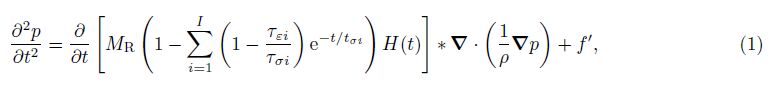
Since density and quality factor change gradually, the reflection is generated mainly by the sudden change of the velocity. The main aim of this paper is to image the velocity perturbation. The relaxation modulus can be expressed by the combination of velocity and density and then Eq.(1)can be expressed as

where f =$\frac{1}{{{v^2}}}f'$, wavefield p and source term f are the functions of spatial location and time, material parameters v, ρ, τ_εi and τ_δi are the functions of spatial location. Independent variables of those functions are ignored for brief.

2.2 Linearization of the Wave Equation

Based on the superposition theory of the wavefield, the total wavefield can be decomposed into background and perturbation wavefields:

where p₀ is background wavefield; and p_s is perturbation wavefield. The background wavefield which is generated by the source and propagates in the background medium satisfies the equation: where v₀ is background velocity. The slowness perturbation is defined as

Substituting Eqs.(3)-(5)into Eq.(2) and applying Born approximation yield the equation that governs the propagation of perturbation wavefield:

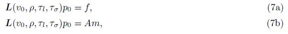
Since Eq.(6)has the same form as the Eq.(4), the perturbation wavefield follows the same laws of the background wavefield. Eq.(6)states that every slowness perturbation acts as a source, but the perturbation wavefield is propagating in the background medium. For brief of following formula derivation, we can write Eqs.(4) and (6)in operator forms:

where A =-$\frac{{{\partial ^2}{p_0}}}{{\partial {t^2}}}$

Auxiliary variables are introduced to solve the equation numerically:

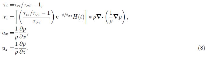
Inserting those definitions into Eq.(2), the new equation for numerical solution can be expressed as

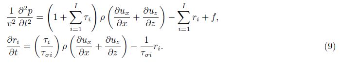
The calculation of time convolution in Eq.(2)which is memory costly is avoided by introducing the auxiliary variable r_i, and calculation of the auxiliary partial differential equations which are easy to solve numerically is needed instead. In another way, the perfectly matched layers(PML)absorbing boundary condition is easier to realize in the new equation because it is first-order derivatives with respect to space variables. Here the complexfrequency- shifted PML(CFS-PML)absorbing boundary condition is used to absorb the outgoing waves.

3 THEORY OF LSRTM IN VISCO-ACOUSTIC MEDIA 3.1 Basic Theory of LSRTM

The imaging method based on inversion is a minimum norm problem. It seeks for the optimal model that minimizes the norm of the differences between forward modeling seismograms and real data. Firstly, a scale product operator(Tanrantola, 2005)in data space is defined as

while the scale product operator in model space is defined as where V(x)is the spatial range of subsurface; t0 and t1 are the starting and terminal times, respectively.

The objective function of LSRTM is defined as

where the first term is the part that minimizes data residual, the second term is model constraint, Wd is the weight function for data residual and Wm is the weight function for the model.

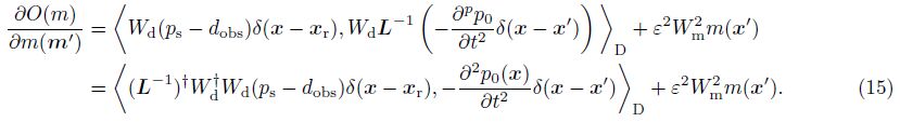
The gradient-based optimal algorithm critically relies on the derivative of the misfit function with respect to the model parameters, i. e. the gradient. The gradient can be derived as

where $\frac{{\partial {p_s}(x, t)}}{{\partial m(x')}}$ is the partial derivative wavefield which can be obtained by differentiating the Eq.(7b)with respect to medium parameter m: The partial derivative wavefield in Eq.(14)is the solution to a new forward modeling problem, driven by the virtual sources at the location x0. The virtual source represents the interaction of the background wavefield with the unit point perturbation of material parameters. Combined with Eq.(13), the gradients exists at those points which can predict seismograms that can best fit the missed reflection.

The partial differential wavefield at each point needs one forward modeling, so it can not afford to calculate gradients using Eq.(13). With the help of adjoint-state method, only one forward modeling and one backward modeling are needed.

Inserting Eq.(14)into to Eq.(13), and using the adjoint operator of the forward modeling operator, the final gradient can be expressed as

The derivation of the adjoint operator refers to appendix A. The adjoint wavefield is defined as

then the gradient can be expressed in a simple form:

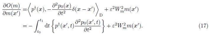
The gradient in Eq.(17)is the zero-lag cross-correlation of the second-order derivative of the background wavefield with the adjoint wavefield which is determined by the backward propagation of the data residual controlled by the adjoint wave propagation operator and the terminal condition. It can be proved that the algorithm is stable. The computational efficiency is also improved because only one forward modeling and one backward modeling are needed to calculate the gradients. Using the steepest descent method, the model can be updated as

where P is the precondition operator. The optimal precondition operator is the inverse of the Hessian matrix, but the heavy computational cost prevents it from using in practical problems. Here we use the energy of the background wavefield to approximate the diagonal element of the Hessian matrix. This precondition operator improves the convergence rate and enhances computational efficiency.

In the visco-acoustic medium, energy of the reflection from deeper reflectors is very weak, so the convergence rate can be improved if some modification is made to gain the weight for the data residual at long time. In addition, some model constraint can be added to stabilize the inversion. Here we use the L1 norm sparse constraint to improve the resolution. It is realized by the iterative reweighted method.

3.2 Phased Encoding Method

Three times of forward or backward modeling are needed at each iteration for the conventional LSRTM. Computational cost of forward modeling based on the linear wave equation is twice that the conventional forward modeling. So the computational cost of LSRTM with N iteration is 2.5N times that the conventional RTM. The high computational cost prevents the method from using in large 2D and 3D models.

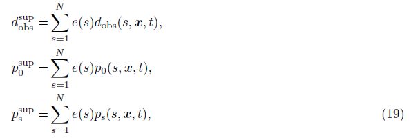
No matter the LSRTM or the conventional RTM, their computational costs are proportional to the number of shots. Similar to the plane wave migration(Yang et al., 2008)multiple shot gathers can be encoded into one supergather by the phase encoding technique. Migration using the supergather can decrease the computational cost effectively. The crosstalk noise introduced can be suppressed by using the dynamical encoding method(Schuster et al. 2011).

The supergather can be constructed by

where s is the shot number; and e(s) is the phase encoding function. Here we use the r and omly generated 1 and -1 as the encoding functions which change r and omly at each iteration. Because the linear relationship between the wavefield and source, one supergather needs only one numerical modeling.

Inserting Eq.(19)into Eq.(17), we have the gradient after using phase encoding:

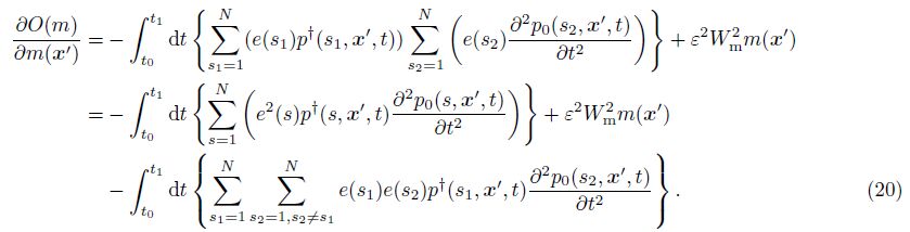
The first term in Eq.(20)is the correct gradient function which is same as the conventional LSRTM, while the second term is the crosstalk noise introduced.

The crosstalk noise is r and om between every iterations because the encoding functions are generated r and omly. So the crosstalk noise is suppressed and true imaging result is enhanced as iteration increases. In addition, when the more supergathers are used simultaneously, the signal-noise-ratio becomes higher. When the number of supergathers is same as the number of shots, the method is reduced to the conventional LSRTM.

4 SYNTHETIC EXAMPLES

The method has been applied to a simple three-layer model and 2D SEG/EAGE salt model to verify its validity. The details of test configurations and analysis are described below.

4.1 Three-Layer Model

The model shown in Fig. 1a consists of three plane layers where the velocity in each layer is 1500, 2000, 2500 m/s and the quality factor is 30, 60, 100, respectively. The size of the model is 150×150, and the sample rate in both directions is 10 m. Synthetic shot records are generated using the linearized wave equation to avoid multiples. In total 150 geophones are deployed on the surface with one geophone at each grid point and 50 point sources are evenly distributed on the surface with a source interval of 30 m. The acquisition geometry is fixed spread, as each geophone is activated for each source. A Ricker wavelet with 20 Hz peak frequency is used as the source wavelet.

The background velocity model is generated by smoothing along both x and z directions. The corresponding relative slowness perturbation model shown in Fig. 1b is calculated by Eq.(5), which can be considered as the ideal imaging result. Both of visco-acoustic and acoustic seismograms are generated for comparison. In Fig. 2, seismic wave dispersion and attenuation can be found easily. The left part of Fig. 2a is the image of visco-acoustic data, while the right part is the image of acoustic data. The data are cut first and then concatenated to plot together. Compared with the acoustic data, the visco-acoustic data attenuate heavily with traveltime differences because of the dispersion. The amplitude spectra of the first reflection waveform from those two data are shown in Fig. 2b. High frequency components of the visco-acoustic data attenuate heavily and the total energy is weak. Mislocation, lower imaging amplitude and low resolution will appear in the imaging result if attenuation and dispersion are not corrected during imaging.

The imaging results using the visco-acoustic LSRTM and acoustic LSRTM are shown in Fig. 3. The imaging result at first iteration shown in Fig. 3a is approximately amplitude-preserved because the precondition operator is applied. Combined with the third line in Fig. 3d, we can find that the imaging amplitude at the center of the model is almost the same as the ideal result, though there are some low wavenumber noise. On both sides of the model, imaging amplitude decreases because of weak illumination. The imaging result after 80 iterations is shown in Fig. 3b. With the increase of iteration, the high wavenumber components of the model are well recovered and the low wavenumber noise is suppressed. Imaging amplitude imbalance caused by weak illumination along the lateral direction is also corrected. From the imaging result comparison shown in Fig. 3d we can find that waveforms of the final imaging result are more close to the real slowness perturbation.

The acoustic LSRTM imaging result is shown in Fig. 3c. This numerical test uses the same data but ignores the influence of the quality factor. Combined with Fig. 3d, we can find that the reflectors are mislocated because of velocity dispersion, and the imaging amplitude is too weak because of attenuation. In addition, some other imaging noises are imported in the acoustic LSRTM imaging result.

4.2 Salt Model

The initial 2D salt model shown in Fig. 4a is a slice of the original 3D SEG/EAGE salt model. This model is used to verify the applicability of the imaging algorithm for the model with high-velocity anomalies. In this paper the quality factor model is constructed according to the Li’s empirical formula(Li, 1993).

There are 780 grid points in lateral direction and 209 grid points in depth direction. The sampling rate is 20 m in both directions. The minimum and maximum velocities are 1500 m/s and 4450 m/s, respectively, and the corresponding minimum and maximum quality factors are 34 and 373, respectively. Viscosity is heaviest near the surface and weakest in the salt dome. The background velocity model is shown in Fig. 4c and the corresponding slowness perturbation which can be regarded as the ideal imaging result is shown in Fig. 4d. Totally 97 point sources are evenly distributed on the surface with a source interval of 160 m. The source wavelet is Ricker wavelet with 10 Hz peak frequency. And 780 geophones are deployed on the surface with one geophone at each grid point.

The first iteration of visco-acoustic LSRTM is shown in Fig. 5a. Similar to the conventional RTM, the imaging result is heavily contaminated by the low frequency noise, especially at the top of the salt dome marked by a dashed ellipse. Although the precondition operator is applied, amplitude imbalance is still present. As shown in Fig. 5b, a part of low frequency noise can be suppressed if a high-pass filtering is applied, but this is no amplitude-preserved process which can damage the relative strength of the imaging amplitude. After high-pass filtering, heavy noises are imported near the source location(dashed rectangle in Fig. 5b) and imaging amplitudes are damaged at the top of the salt dome(dashed ellipse in Fig. 5b). In addition, both imaging amplitude and resolution are lower because of attenuation. The imaging result after 50 iterations is shown in Fig. 5c. Through iterative inversion, not only the low frequency noise is suppressed, but also the imaging amplitude is balanced. The resolution is also higher than the conventional RTM. From the curve comparison plotted in Fig. 6, we can find that imaging result almost completely agrees with the true slowness perturbation. It demonstrates that our visco-acoustic LSRTM is a true-amplitude imaging method.

The imaging result has a high resolution expect the regions marked by dotted boxes in Fig. 5c. Too weak illumination is the main reasons for the poor imaging result. At the top surface of the salt dome marked by the first dotted box, most of the reflections propagate outside the model and only a few reflections can reach receivers. For the area below the salt dome, the salt dome can be seen as a shield to prevent the seismic waves from propagating downward and upward. The area marked by the second dotted box has the weakest illumination, so it is hard to image.

The imaging method based on inversion can compensate for illumination shadow, but those almost blind areas cannot be imaged. Proper artificial constraints can be used to help improve the imaging result. The imaging result using the acoustic LSRTM is also plotted in Fig. 5d to validate the importance of considering viscosity. The input shot gather and other parameters are same as the visco-acoustic LSRTM. The only difference is the quality factor is infinity. Compared with Fig. 5d, we can find that the imaging result has low signal to noise ratio(SNR), low resolution and under-estimated imaging amplitude.

The different phenomena of wave propagation in acoustic and visco-acoustic medium are the main reason for the enhancement of the imaging noise. It is difficult to find a acoustic model which can generate shot gathers that fit the visco-acoustic shot gathers. It is more serious for the shallow and long offset data. For quantitative comparison of the imaging resolution, we calculate the average wavenumber spectrum which is the stack of the wavenumber spectra in depth direction. The average wavenumber spectra of acoustic LSRTM, visco-acoustic LSRTM and the true slowness perturbation are plotted as trace 1, 2, and 3, respectively in Fig. 5e. Although average wavenumber spectrum only reflects the resolution in depth direction, it provides us a way to measure the resolution. The visco-acoustic LSRTM recovers the high wavenumber components of the model effectively, so the average wavenumber spectrum is closer to the true one. The effective b and width of the average wavenumber spectrum for the acoustic LSRTM is narrower than the others, so acoustic LSRTM imaging result has the lowest resolution. The imaging curve at locations A and B in Fig. 5c and 5d are plotted in Fig. 5f. Comparison in Fig. 5f indicates that the imaging amplitude is under estimated and the resolution reduces if the viscosity of the medium is ignored during migration.

Through the above analysis, we can find that it is necessary to consider the viscosity of the medium during migration. And the visco-acoustic LSRTM has several advantages, such as suppressing the imaging noise, compensating for attenuation, higher imaging resolution, and providing true-amplitude imaging result. The main disadvantage of this method is the heavy computation cost. Here we use the phase encoding technique to reduce the computational cost.

LSRTM with phase encoding is also tested here to verify the ability of improving computation efficiency. The imaging result with one supergather is shown in Fig. 7. The imaging result at 10th iteration shown in Fig. 7a is heavily contaminated by the crosstalk noise and has a low SNR. Difference between image results using phase-encoding and conventional LSRTM at 10th iteration is shown in Fig. 7b. The crosstalk noise has the same magnitude with the imaging result. With the increase of iteration, the crosstalk noise is suppressed gradually. The imaging result at 100th iteration shown in Fig. 7c is almost same as the imaging result by the conventional LSRTM at 50th iteration. This can be verified by the difference profile shown in Fig. 7d. Although those imaging results are almost same, the computational cost is only 0.0206 times that of the conventional LSRTM. The LSRTM with phase encoding can improve the computation efficiency heavily.

Multiple supergathers can be used simultaneously to suppress the crosstalk noise when we run the program on PC-cluster with the MPI environment. When the number of supergathers is the same as the number of shot gathers, the method is reduced to the conventional LSRTM. Imaging results at 10th iteration using 4, 8 supergathers are shown in Fig. 8. Combined with Fig. 7a, we can find that the crosstalk noise is suppressed gradually with increase of the number of supergathers. Suitable schemes can be selected according to actual situations.

5 CONCLUSIONS AND DISCUSSION

A visco-acoustic LSRTM method in the time domain is proposed in this paper. Compared with the conventional inverse Q migration, this method has the following advantages:(1)It can compensate for the attenuation while avoiding the instability problem.(2)It can provide true-amplitude imaging result.(3)It can suppress imaging noise effectively and compensate for illumination shadow. And(4)with the help of phase encoding technique, the computational cost can be reduce to the same level as the conventional RTM.

The method presented in this paper is based on the GSLS model and is restricted in 2D, but it can be easily extended to other models and 3D. Compared with the method in the frequency domain, the method is easier to implement with help the modern high-performance computer.

Although the method described here is based on complete theory and is verified by a synthetic data test, there are a series of challenges to overcome when real data are processed. These difficulties include:(1)Amplitude-preserved pre-process and evaluation. The pre-processes mainly include de-noising, consistent correction of source energy, removal of the surface wave and other elastic effects.(2)High-precision macro-velocity estimation and quality factor extraction. Since the method is very sensitive to accuracy of background velocity and quality factors, large imaging errors or even divergence will happen if the error of material parameters is large. All the true amplitude imaging and waveform inversion methods will face the first problem which involves a wide range of techniques. Here we do not consider it too much. The second problem is how to obtain accurate background material parameters. We think the following aspects should be considered:(1)Establish a reasonable workflow for imaging the different range of wavenumber components of the subsurface model. The low wavenumber components can be imaged by tomography, migration velocity analysis or the Laplace-domain waveform inversion. The medium-wavenumber components can be imaged by frequency or time domain waveform inversion. And high wavenumber components can be imaged by the LSRTM. Different ranges of wavenumber components can be gradually imaged uisng different methods, and finally an accurate subsurface image is generated. Overall, LSRTM can be seen as a linear waveform inversion that can image the high-wavenumber components of the model.(2)The near-surface model should be finely constructed, especially the quality factor model. This is the most import part when processing onshore seismic data. The complex near surface structure has important influences on seismic wave propagation and the imaging result. The firstarrival traveltime tomography or the finite frequency tomography is the main tool to inverse the near surface velocity, but it is difficult to inverse the quality factor. First arrival waveform inversion may be an important tool to inverse velocity and quality factor jointly.(3)Adding some constraints to LSRTM may be a good choice to make the method stable. Those constraints can come from well log data, previous geological information and other sources. In a word, the inversion method based on waveform fitting has irreplaceable advantages in theory, but in real data processing, some other matching techniques and a more stable LSRTM method should be developed. These will be the next focus of our work in the future.

6 Appendix A: Derivation of Adjoint Visco-Acoustic Wave Equation Operator

With the definition of scale product operator in data space in Eq.(10), the adjoint operator satisfies

where L is the wave equation operator; p is the wavefield controlled by the wave equation operator; L^† is the adjoint wave equation operator; and 1^† is the adjoint wavefield controlled by the adjoint wave equation operator.Inserting the wave equation operator to Eq.(A1)yields

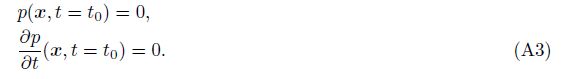
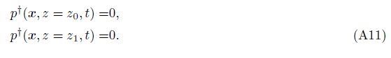
The boundary condition and initial condition for the wave equation should be defined before derivation. The medium is supposed to be in equilibrium at time t = t0, i.e. stress and its derivative are zero everywhere in the medium:

If the free surface is considered, then the boundary condition at the top surface is If the free surface is not considered, then the range of medium is assumed to be infinite. The Sommerfeld radiation condition is applied:

We start the derivation with the first term on the right-h and side of Eq.(A2). Repeating integration by parts yields

By imposing the terminal conditions, there are

We can obtain the first ingredient of the adjoint operator:

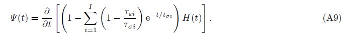
The relaxation rate function ψ(t) is defined to simplify the derivation related with the second term of the right-h and term:

Taking z direction as the example to show the derivation, exp and ing the convolution and repeating integration by parts yield

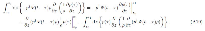
We impose the boundary conditions

Thus, the first two terms in Eq.(A10)are forced to be zero: When free surface is considered, Eq.(A11)is a free surface boundary condition; if not, Eq.(A11)is an absorbing boundary condition.

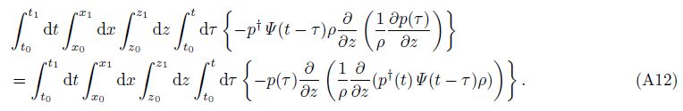
With the help of identity $\smallint _{{t_0}}^{{t_1}}\left\{ {\smallint _{{t_0}}^{{t_{}}}d\tau } \right\}dt = \smallint _{{t_0}}^{{t_1}}\left\{ {\smallint _\tau ^{{t_1}}dt} \right\}d\tau $, we can change the order of integration and interchange the symbols:

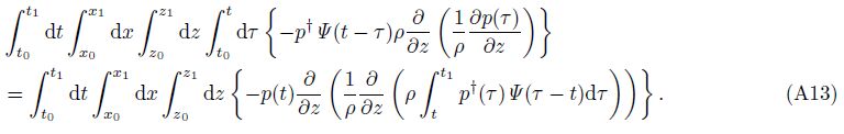
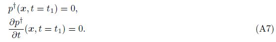
The anti-causal function ψ^† is defined which satisfies

Combining Eqs.(A13) and (A14)yields In the same way, the derivation in the x direction is

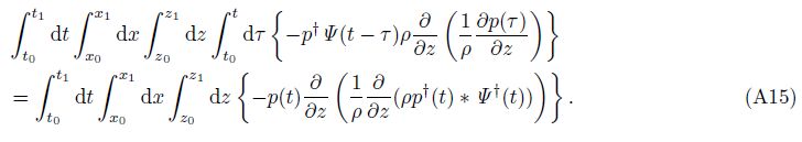
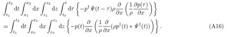
Inserting Eqs.(A8), (A15), and (A16)into Eq.(A2), we obtain the adjoint wave equations

where the right-h and term is the source term. Inserting the detail description of ψ^† into Eq.(A17)yields The adjoint wave equation has the approximate form with original wave equation(Eq.(2)), so it can be solved with the same numerical method.

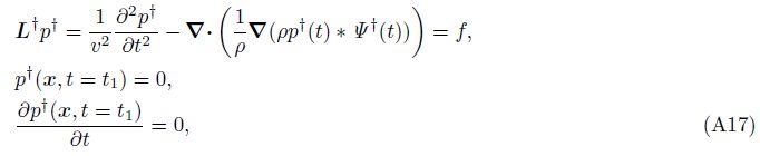
It can be proved that the forward wave propagation based on the adjoint wave equation is unstable, but the backward wave propagation using the terminal condition(A7)is stable. The stability problem is avoided through the introduction of the adjoint wave equation.

7 ACKNOWLEDGMENTS

We thank two anonymous reviewers for their comments and constructive suggestions that led to significant improvements of the manuscript. This work was supported by the National Natural Science Foundation of China(40974073), National High-tech R&D Program of China(863 Program, 2011AA060301) and the Fundamental Research Funds for the Central Universities(13CX06014A).