 2014, Vol. 57


2. Key Laboratory of Earthquake Monitoring and Disaster Mitigation Technology of CEA, Guangzhou 510070, China;
3. Key Laboratory of Earthquake Early Warning and Safety Diagnosis of Major Projects of Guangdong Province, Guangzhou 510070, China
The most basic data in seismology is the continuous waveform data recorded by seismographs. Such data records reveal the actual ground motion to a certain extent at the observation site. But these records of ground motion are incomplete and contain distortion because of limited frequency characteristics of an actual seismic observation system. In order to study the true ground motion, it is necessary to make data processing on instrument response elimination, which is just the deconvolution process of transfer function. To study some specific signals, the frequency b and of recorded data may also need to be further restricted. Therefore recovering true ground motion from actual data records and simulation processing of different instrument types have both basic and practical significances.
Processing methods for eliminating instrumental effect have been summarized into four groups by Aki and Richards(1980). Two of them are carried out entirely in the time domain, the other two need to be conducted in the frequency domain. For the approach integrating directly from the seismometer differential equation, some simplified assumptions and additional restrictions should be applied to the distribution pattern of recorded data and integral initial conditions, due to the presence of errors and disturbances in the data recorded(Wang G F, 1986). Methods in the frequency domain calculating with high computational efficiency may produce high-frequency and very low frequency spectral distortions easily(Aki and Richards, 1980; Li H J, 1992a, 1992b). Li(1992a, 1992b)had proposed a “reference cycle” approach to modify the spectrum in order to reduce the distortion caused by instrumental correction. He simulated instrumental records and verified the results of instrumental correction with the approach of solving state equation with modern control theory, and had achieved good results. Li’s method may really improve the estimate of ground displacement. Although Li’s method works well, its algorithm is too complicated to be applied to conventional data processing in routine work. Liu et al.(1997)still preferred to conduct long-period and mid-long period seismograph record simulation with direct Fourier analysis.
The fourth method mentioned by Aki and Richards(1980)is to apply a recursive filter. They pointed out that if only a small amount of the recursive filter coefficients are required for a given purpose, this filter is more efficient than the FFT method. The situation is not simple in practice, because the real seismic observation system usually cannot be completely described by a recursive filter with a small amount of coefficients. Nevertheless, it becomes possible in the case that low frequency characteristics of a seismometer are primarily considered and errors caused by ignoring high frequency effects are acceptable. For an inertia seismometer model, Wang(1986)deduced a second order recursive filter, which obtains the response of an inertial mass to the ground displacement. It is easy to show, see Section 2 below, that this filter is applicable to the output of a velocity-flat-response seismometer sensing ground velocity. By using this method, the recovery of ground velocity from modern seismic velocity records and alternate velocity records simulation in turn may be achieved. Since this filter includes three recursive coefficients associated with the ground motion, two of which deal with lagged historical data, the recovery process requires two initial values to be assumed and three ones should be assumed for simulation on the other h and .
Some traditional analog seismographs contain electronic amplifiers and other galvanometer components. Their transfer functions are more complex than a conventional inertia seismometer model. Some practical work, magnitude calculation for example, need to simulate traditional instrumental records from modern seismographic records. Wang et al.(2006)has deduced recursive filters for simulation of DD-1, DK-1 seismographs by bilinear transformation.
With the rapid development of strong ground motion observation techniques, the corresponding data processing method has also been developed rapidly, including various types of simulation methods on ground motion response. Jin et al.(2003)have done detailed researches on the four more representative kinds of these simulation methods and deduced their recursive filters(Jin et al., 2004). They tried to simulate ground velocity records in real time from acceleration records and integrate them into a weak motion seismograph network.
In this paper, an alternative recursive filter is presented to achieve seismogram deconvolution and simulation. Only one of its coefficients involves ground motion data. Hence, no initial values about ground motion should be assumed in the deconvolution procedure, and only one needs to be assumed in the simulation procedure. Instances using this filter in numeric experiments and practical applications are given below. The simulated result is velocity record in this case. On the other h and , the physical quantity obtained in the deconvolution operation is different from previous work.
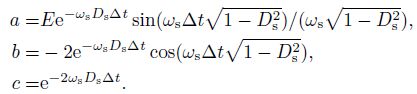
2 RECURSIVE FILTERThe transfer function to the ground displacement of an inertial seismometer can be written as(Wang, 1986)


Let us now consider the ground acceleration changing rate with time, which is denoted as w(t)= d3x/dt3. Applying Laplace transformation to it yields W(s)= s3X(s). Then the transfer function to w(t)is


Since impulse invariance method may bring in spectrum aliasing(Oppenheim and Schafer, 1980), sufficiently b and -limited data is required in the application of filter represented by Eq.(6). This requires that the seismic observation system includes a b and -limited seismometer or a data acquisition system with a proper low-pass filter. All the data recorders used in this work satisfy this requirement for their embedded low pass filter with stop-b and attenuation over 130 dB. Hence no spectrum aliasing happens in this work.
In addition, cares must be taken on the physical meaning of Eq.(6). The quantity obtained in deconvolution operation on velocity data corresponds to the changing rate of ground acceleration with time rather than ground displacement, velocity or acceleration that we usually deal with.
Suitability and effectiveness of the recursive filter are illustrated in three aspects using examples of a numeric experiment, actual event simulation and relative orientation measurement of seismometer discussed in detail below. Information of all seismometers used in this work, including their model names, working b and s, manufacturers, serial numbers and so on, is listed in Table 1.
| Table 1 Seismometer informations |

According to the principle of seismometer calibration, the calibration event corresponds to that the seismometer is sensing an equivalent ground acceleration procedure which is proportional to the calibration source signal. By applying the recursive filter described in the previous section to a calibration response record, the deconvolution operation will generate a data series corresponding to the source signal changing rate with time and the source signal may be recovered after numerical integration. However, there should be environmental noises in the actual data.
A pseudo r and om binary signal(PRBS)is one of the commonly used excitation signals for electrical calibration(Berger et al., 1979). Since a PRBS is easy to implement and has spectral characteristics close to white noise, a complete transfer function may be estimated from a calibration using PRBS. Signal mutation occurs between the symbol 0 and 1 in a PRBS, while other times the signal remains unchanged. So its time derivative should be a δ function at the time PRBS symbol changing between 0 and 1. Therefore, PRBS should be a good choice for the numeric experiment with the filter described in the previous section.
The basic contents of numerical experiments in this work are: deconvolution operation is performed on the PRBS calibrating response record of a very broad b and seismometer to yield a series of equivalent ground acceleration rates changing with time, the series is then used as input to simulate the response of the broad b and seismometer, and the simulated response is compared to real calibrating response of a true broad b and seismometer finally.
Deconvolution and integration results for a PRBS calibrating response record using No.1 very broad b and seismometer listed in Table 1, which was connected to a EDAS-24IP3 data recorder manufactured also by Geodevice at Beijing are shown in Fig. 1. To show details clearly, just foremost 1000 samples are drawn for illustration. The original PRBS in the figure is a record of separately sampled calibrating output of the recorder. It is obvious that the deconvolution results include a series of sharp pulse close to δ function, which is consistent with the expectation. The recovered PRBS via integrating once is also well consistent with the original PRBS but with absence of some high frequency elements caused by the fact that high frequency properties of the seismometer and low-pass filter of the recorder are neglected in the deconvolution process.

|
Fig.1 Deconvolution results of PRBS calibration response |
Instruments of two operating stations in the Guangdong regional seismographic network were chosen to do the simulation experiment. Their seismometers are No.2 combination listed in Table 1 with EDAS-24IP3 data recorders made by Geodevice. Calibration using PRBS was conducted at each station with the same parameters: series code bin10r, symbol element width 200 ms, signal amplitude 900 counts, and series repeated once. The calibration response of 120 second period very broad b and seismometer was then simulated to response of a 60 second period broad b and seismometer after deconvolution.
The actual and simulated waveform records are shown in Fig. 2a. It is easy to see that the simulated record is well consistent with the actual response of BBVS-60. The different response post calibrating signal should be the effect of different offset current in the calibrating circuit between two seismometers. Corresponding spectrum results are shown in Fig. 2b. The simulated spectrum coincides basically with the actual one of BBVS- 60 response. Numerical experiments of deconvolution and simulation validate the suitability of the recursive filter presented in the previous section, which has a clear physical meaning and may yield results comparable to a real measured signal.

|
(a) BBVS real & simulated response of PRBS calibration; (b) Spectra of BBVS real & simulated response. Fig.2 Real and simulated results of PRBS calibration |
A JCZ-1T ultra broad b and seismometer is running at the Guangzhou seismograph station(see combination No.3 in Table 1). It is connected to an EDAS-24IP6 recorder made by Geodevice. DS-4A short period seismometer of the combination was mounted temporarily at the same site with a TDE-324CI recorder made by Taide at Zhuhai, Guangdong. Both systems have recorded at the same time the earthquake of M7.3 on 31 August 2012 in the Philippine Isl and s. The BB channel record of JCZ-1T is simulated to short period one using the filter described in Section 2. The result is consistent with the actual record of DS-4A except the different input scales of recorders. The UD component is shown in Fig. 3.

|
(a) JCZ-1T UD ultra broadband record; (b) Simulated SP record; (c) DS-4A UD real SP record. Fig.3 Real and simulated earthquake records |
In practice, seismic observation in a borehole can suppress ambient noise to improve SNR effectively, but orientations of its horizontal sensors are not easy to determine. If there is a base with locking capability preinstalled at the bottom, the orientation can be measured with a downhole gyro. But a downhole gyro is expensive and vulnerable, so that many downhole seismographs are installed without measurement of orientation with a gyro. A compromise approach is to install a seismometer at the ground surface near the wellhead simultaneously and to estimate the relative orientation with correlation analysis. Sometimes it is also necessary to relatively orientate a seismometer mounted at the ground surface. Lü et al.(2007)have shown in detail the correlation analysis method to estimate seismometer orientation relatively. Güralp System Ltd has integrated this method in the software product Scream(4.2 and later versions), and the software product SMARTAngle of Geotech also provides the same analysis function. Both pieces of software calculate correlations between the NS component of the reference seismometer and the rotating horizontal components of the other seismometer, and find the best fit results. Due to the fact that there may be some slight errors in the orthogonality of the actual horizontal sensors and the more important that noises present in the recorded data, correlation analysis made on both horizontal components may yield different angle results. Hence, Lü et al.(2007)recommend to take the mean value of both horizontal component analyses.
The method introduced by Lü et al. is different from that introduced by Holcomb(2002). The difference does not exist in their algorithms, but only in the ways to express their results. Holcomb showed his results in a polar plot which caused overlay of negative and positive correlation values. This made that Holcomb could not recognize the correct sensor orientation from his result plotting. In contrast, Lü et al. plotted their results in a Cartesian coordinate system which showed negative and positive correlation values via rotation angles correctly.
The data sample length for their correlation analysis was not mentioned in the paper of Lü et al., and Holcomb used just 256 points of partially overlapped data samples in his coherence analysis for downhole observed records. Lü et al. and Holcomb both mentioned that r and om noise except microseism is harmful to the correlation analysis. Therefore, longer sample records, with sample rate of 100 sps and one hour long for example, are chosen in analysis in this work to reduce the influence of r and om noise to ensure good stability and consistency.
When the tested seismometer works in a frequency b and different from the reference one, Lü et al.(2007)just suggested to filter data records with the same b and that both seismometers respond flat. However, according to practical experience, just filtering with the common b and in this case may not be able to achieve good results. Hence, the recursive filter in Section 2 is tried to simulate a record with consistent narrower b and from data recorded with a broader b and sensor and then do the common b and filtering. Multiple experiments using several seismometers with different b and s are done in this way and have achieved good results. Two among them with seismometer orientation measured absolutely with instrument are discussed in detail below. Both experiments are done on a combination of a broadb and seismometer with period of 60 seconds and a short period one with period of 2 seconds, but these two broadb and seismometers are products of different manufacturers. Correlation analyses are conducted on the same data pairs with and without simulation. Taking into account the working frequency b and of short period seismometers, data records are filtered with a 0.5~5.0 Hz b and of frequency. The absolute orientation measurement instrument used in this work is a north finder model NV-NF301 made by NAV Technology Co. Ltd at Beijing with a power tuning gyro inside which makes its measurement insensitive to environment magnetic fields. It can find north in the range of 0°~360° with an accuracy of 0.3° and a resolution of 0.01°. Each orientation angle is measured several times and an average value is taken to reduce errors.
The first experiment is done on the No.4 combination of seismometers in Table 1. They are connected to an EDAS-24GN6 recorder made by Geodevice with sample rate set to 100 sps, filter mode set to minimum phase and input scale set to ±10 V. Both seismometers are mounted just 50 cm apart from each other on the same pier. Orientations measured by the north finder are 317.7° for T34294 and 350.4° for 09178 separately with a difference of 32.7°. For the analysis without simulation, calculation on EW reference component achieves a maximum correlation coefficient of 0.9761 when the tested sensor is mathematically rotated to the angle of 34.0° while on NS achieved maximum of 0.9744 at 33.5°; the mean value is 1.05° apart from result of north finder. Fig. 4a shows the result of correlation in a 4° rotation step and Fig. 4b illustrates the detailed result around the maximum correlation coefficient in a fine 0.1° step. Filtered detailed waveforms before and after rotation at the optimum angle are shown in Figs. 4c, 4d, 4e, and 4f separately. For the analysis with simulation, calculation on EW component achieved maximum of 0.9993 at 33.1° while on NS achieves maximum of 0.9989 at 32.7°; the mean value is 0.2° apart from result of north finder. Fig. 5 shows results corresponded to Fig. 4. It is obvious that with simulation, the correlation coefficient is higher, the rotated waveforms conform better and the rotation angle is more close to the value measured with north finder. In short, the simulated results are better than that without simulation.

|
(a) Raw correlation coefficients; (b) Fine correlation coefficients; (c) Original EW data; (d) Original NS data; (e) Rotated EW data; (f) Rotated NS data. Fig.4 Correlation results of T34294 vs 09178 without simulation |

|
Fig.5 Same as Fig. 4, but for correlation results of T34294 vs 09178 with simulation |
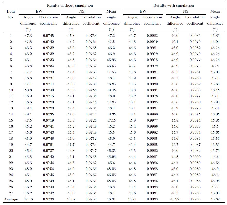
The second experiment is done on the No.5 combination of seismometers in Table 1. They are both connected to an EDAS-24IP6 recorder also made by Geodevice with parameter setting consistent with the previous experiment. Both seismometers are also mounted 50 cm apart from each other on a single pier. Orientations measured by the north finder are 251.4° for 08200 and 206.3° for 11M46 separately with a difference of 45.1°. Experiment data collection is lasted 27 hours continuously. Analyses are conducted on each hour record and results are listed in Table 2. Figs. 6 and 7 show results of first hour data analysis corresponded to Figs. 4 and 5. All results reveal that correlation coefficients calculated with simulation are higher than those without simulation. Angle results for calculations without simulation are scattered from 44.7° to 50.6° with an average of 46.9°. On the other h and , angle results for calculations with simulation are distributed only from 45.4° to 46.3° with an average of 45.8°, which are more close to values measured by the north finder.
| Table 2 Correlation results of second experiment on pier |

|
Fig.6 Same as Fig. 4, but for correlation results of 08200 vs 11M46 without simulation |

|
Fig.7 Same as Fig. 4, but for correlation results of 08200 vs 11M46 with simulation |
Based on the above results, under the experimental conditions, correlation analyses with simulation on two seismometers with different frequency b and s can achieve more reliable and less erroneous results.
Additional experiments are conducted at Shiliugang Station(SLG in short), a working station in Guangdong regional seismographic network, with a borehole observation system made by Güralp and the results are consistent with the orientation given by the manufacturer while system installation. Seismometer information is listed as No.6 and 7 combinations in Table 1. The downhole seismometer is installed at a depth about 220 m. Its orientation is measured with surface seismometer correlation method integrated in Scream of Güralp and is set into the CMG-DM24 recorder to rotate the output signals. The surface sensor is aligned north using a compass. So, the rotated NS outputs may be thought as records in the geomagnetic NS direction. There are piers poured on bedrock in the basement about 15 m below surface at a distance of about 100 m from the wellhead.
The BBVS-60 seismometer of No.6 combination listed in Table 1 was first mounted at the surface about 1.5 m away from the wellhead. It was oriented using the north finder and connected to an EDAS-24IP3 recorder synchronized to GPS. The surface system recorded signals with the same sample rate of 100 sps as the downhole system. Five data segments, with half an hour length each, were used in correlation analysis. The CMG-3TB borehole system records were analyzed with and without simulation separately. According to the microseism period, about 2~3 s, in the Guangdong area, frequency b and 0.2~0.6 Hz was applied in the filtering process. The resulted average orientation differences are -0.17° with simulation and -0.43° without simulation as shown in Table 3. The angle is counted positively for clockwise deviation of the downhole CMG-3TB seismometer orientation from the geographical north. Orientation results without simulation are close to those with simulation in this experiment, but correlation coefficients with simulation are a little higher than those without simulation.
| Table 3 Microseism correlation results of downhole records |
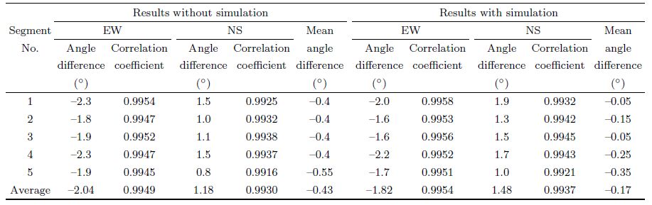
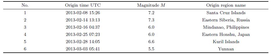
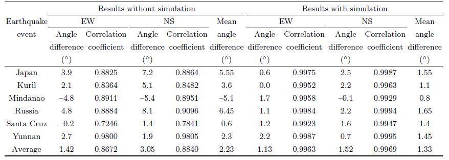
The CMG-40T seismometer, another product of Güralp, of No.7 combination in Table 1 was then mounted on a pier in the basement. It was also oriented using the north finder and connected to an EDAS-24GN3 recorder synchronized to GPS with the same sample rate of 100 sps. This system ran there for nearly one month and had recorded coincided with the borehole system some teleseisms occurred in different directions. Six events recorded clearly were chosen for correlation analysis and they are listed in Table 4. Event parameters are taken from the earthquake catalog released by China Earthquake Networks Center. The CMG-3TB borehole system records were also analyzed with and without simulation separately. Filter b and was chosen according to event spectra in two cases: for the Yunnan earthquake with a smaller epicentral distance but relative abundant high frequency components, a pass b and of 10~2 s was used; and a pass b and of 15~5 s was used for the other five events. The resulted average orientation differences are 1.33° with simulation and 2.23° without simulation, respectively(Table 5). It is obvious that the analysis results without simulation are more largely scattered and the correlation coefficients are even much lower than those with simulation.
| Table 4 Earthquake events information |
| Table 5 Earthquake correlation results of downhole records |
According to the results of numerical experiments and real event simulation, this paper analyzes application limitations and effects using the recursive filter. The conclusions are as follows:
(1)The suitable conditions for applying this method are the requirement of b and limited data or errors caused by ignoring high frequency effects are acceptable.
(2)This recursive filter includes less coefficients than that designed by bilinear transformation, and its usage is more convenient.
(3)The quantity obtained in deconvolution operation on velocity data records corresponds to the changing rate of ground acceleration with time.
(4)The operations are conducted in the time domain, and a few initial values should be assumed. Reasonable assumptions can be made easily from the actual observation environment. The operations are not easy to lead to distortions from the assumptions unlike that, in the frequency domain, the analysis without or with inappropriate modification on the spectra may lead to long-period distortions easily(Li, 1992a, 1992b).
In summary, with full attention to the applicable conditions and the physical meaning of the results, the application of this method is easy to achieve satisfactory results from deconvolution and simulation.
7 ACKNOWLEDGMENTSThe author thanks his colleagues who participated in the experimental work at the SLG seismograph station, including Lin Wei, Lao Qian, Chen Jiantao, Wang Guowang, Huang Yong and Jia Yu. The author also thanks Yang Dake of Institute of Geophysics, CEA and two anonymous reviewers, who have given valuable and useful suggestions which made this paper enriched in many ways.
| [1] | Aki K, Richards P G. 1980. Quantitative Seismology Theory and Methods. Vol. II. San Francisco:W H Freeman and Company, 584-585. |
| [2] | Berger J, Agnew D C, Parker R L, Farrell W E. 1979. Seismic system calibration:2. Cross-spectral calibration using random binary signals. Bull. Seism. Soc. Am., 69(1):271-288. |
| [3] | Holcomb L G. 2002. Experiments in seismometer azimuth determination by comparing the sensor signal outputs with the signal output of an oriented sensor. U. S. Geol. Surv. Open-File Rept. 02-183. |
| [4] | Jin X, Ma Q, Li S Y. 2003. Comparison of four numerical methods for calculating seismic response of SDOF system.Earthquake Engineering and Engineering Vibration(in Chinese), 23(1):18-30. |
| [5] | Jin X, Ma Q, Li S Y. 2004. Real-time simulation of ground velocity using digital accelerograph record. Earthquake Engineering and Engineering Vibration(in Chinese), 24(1):49-54. |
| [6] | Li H J. 1992a. Examination of broadband seismic records recovery of CDSN in the frequency domain with the principle of modern control theory. Acta Seismologica Sinica(in Chinese), 14(1):90-99. |
| [7] | Li H J. 1992b. Determination of the ground displacement using FFT and modern control engineering. Chinese J. Geophys.(in Chinese), 35(1):37-43. |
| [8] | Liu R F, Chen P S, Dang J P, et al. 1997. The application of imitation for broad band digital seismic recording.Seismological and Geomagnetic Observation and Research(in Chinese), 18(3):7-12. |
| [9] | Lü Y Q, Cai Y X, Cheng J L. 2007. Orientation for seismometer with coherence analysing method. Journal of Geodesy and Geodynamics(in Chinese), 27(4):124-127. |
| [10] | Oppenheim A V, Schafer R W. 1980. Digital Signal Processing(in Chinese). Beijing:Science Press, 146-150. |
| [11] | Wang G F. 1986. Calibration and Checking of Seismograph Systems(in Chinese). Beijing:Seismological Press, 255-271. |
| [12] | Wang H T, Chen Y, Zhuang C T. 2006. A method on construction of real time seismic waveform emulation filter with bilinear transformation. Seismological and Geomagnetic Observation and Research(in Chinese), 27(1):68-73. |