1 INTRODUCTION

Magnetotellurics (MT) is a very popular electromagnetic geophysical method of imaging the earth’s subsurface. In recent years Chinese researchers have made some progresses on study the electrical structure of lithosphere by MT^[1,2,3,4]. In 2005 Wanamaker^[5] elaborated on the importance of electrical anisotropy in the electrical modeling and geodynamics,and elucidated the existence of electrical anisotropy in the earth. The two-dimensional (2D) modeling of MT electrical anisotropy is realized with some numerical methods,among which the finite element method (FEM) and the finite difference method (FDM) are mostly applied^[6]. Early in 1975,Reddy and Rankin^[7] did some pioneering work on 2D modeling of electrical anisotropy by solving partial differential equations with FEM. Their work promoted the development of anisotropic theory and has made great influence on other researchers. After 2000,some successful anisotropic experiments of MT data are conducted by the general ideas which are adopted from Reddy and Rankin. Xu (1985)^[8] calculated the MT field on 2D anisotropic geoelectric section by FEM,and his work is the primary study on electrical anisotropic theory in China. Li (2002)^[9] presented the FEM formula for computing the electromagnetic induction on 2D anisotropic geoelectric structure. The FEM was used to solve a coupled system of two partial differential equations for the strike-parallel field components E_x and H_x. Then the resulting system of linear equations was solved by a preconditioned conjugate gradient method. The strike-perpendicular field components E_y and H_y were calculated by numerical differentiation of E_x and H_x afterwards. Subsequently,the results were compared with the previous results of Pek (1997)^[10],which proved the theory of this FEM formula. In 2008,Li^[11] developed this FEM method by using an adaptive unstructured mesh finite element procedure,and managed to improve the quality of numerical solutions. Based on the theory of Reedy (1975)^[7],Pek (1997)^[10] developed some scholars’ work (Haak et al.(1972)^[12],Brewitt-Taylor & Weaver (1976)^[13],$\overset{\lower0.5em\hbox{$\smash{\scriptscriptstyle\smile}$}}{C}$erv & Praus (1978)^[14]) by introducing the finite-difference methods for isotropic electrical media into anisotropic situations. This idea of using FDM to solve partial differential equations showed great effect on the 2D modeling of MT electrical anisotropy.

2 TWO-DIMENSIONAL FORWARD MODELING THEORY OFMT ELECTRIC ANISOTROPY

This paper applies the FDM to the 2D forward modeling of MT electrical anisotropy,which refers to the study of Pek (1997)^[10].

In right-handed Cartesian coordinates (x,y,z),we assume a traditional 2D geoelectric model with its structural strike parallel to the x-axis. The z-axis is positive downwards. The model consists of a finite system of homogeneous,but in general anisotropic 2D blocks. The earth’s surface is assumed to be planar and to coincide with the coordinate plane z = 0. Above the surface (z < 0) a perfectly insulating air layer is assumed. The primary electromagnetic field is modeled by a monochromatic electromagnetic plane wave (angular frequency ω = 2π/T ,with T (unit: second) being the period) propagating perpendicularly to the earth’s surface from sources located at z → -∞.

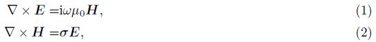
Assume that all media are linear and have electrical properties independent of time,pressure or temperature. In the quasi-stationary approximation,the governing Maxwell’s equations for the electromagnetic field can be written as:

where e^-iωt is a time factor and σ is electrical conductivity tensor. By virtue of the 2D condition ∂/∂x = 0, Eqs.(1) and (2),written for the individual components,reduce to

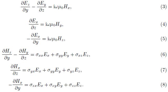
From Eq.(3) to (8),the field components E_y,E_z,H_y and H_z can be calculated by E_x and H_x. Then we can get a coupled pair of second-order partial differential equations for E_x and H_x.

For the TE mode,there is

For the TM mode,we have

In Eqs.(9) and (10),there is

Using the finite-difference method to solve the governing Eqs.(9) and (10): The structure is projected onto a numerical grid and,within a finite grid region,subdivided into a system of electrically homogeneous,but in general anisotropic,rectangular grid cells. The grid is in general irregular and should both fit the geometry of the model and meet general rules accepted for designing numerical grids in modeling for isotropic media.

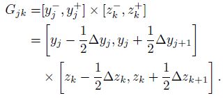
Following $\overset{\lower0.5em\hbox{$\smash{\scriptscriptstyle\smile}$}}{C}$erv and Praus (1978)^[14],we use the integro-interpolation method to derive the FD equations for individual grid notes. In Fig.1 the black solid circle denotes the node point (j,k),and the shadow area denotes the rectangular integration cell G_jk around the node (j,k). And Eqs.(9) and (10) are integrated across the cell G_jk,say

Eq.(9) represents another form of (6),with the y and z field components eliminated by making use of the other equations. The corresponding integral form of this equation,representing the x-projection,is where Γ(G_jk) is the oriented boundary of the integration cell G_jk,dg is the element of the integration path along this boundary,dG = dGe,with e_x denoting the unit vector in the x-direction and dG denoting an areal element of G_jk,which can be written as where ${{\overline{\left( \frac{\partial {{E}_{x}}}{\partial z} \right)}}_{KL}}$ is the mean value of the function $\frac{\partial {{E}_{x}}}{\partial z}$ across KL,and so on for the following ${{\overline{\left( \frac{\partial {{E}_{x}}}{\partial y} \right)}}_{LN}}$,${{\overline{\left( \frac{\partial {{E}_{x}}}{\partial z} \right)}}_{NM}}$,${{\overline{\left( \frac{\partial {{E}_{x}}}{\partial y} \right)}}_{MK}}$,$\overline{KL}$ is the distance between the corresponding vertices of the integration cell (oriented positive counter-clockwise when looking from the positive x-direction,S(G_jk) is the area of the integration cell,j_x is the x-component of the current density,j_x = (σE)_x = σ_xxE_x + σ_xyE_y + σ_xzE_z and ${{\overline{({{j}_{x}})}}_{{{G}_{jk}}}}$ is the mean value of the j_x across G_jk. Approximating the mean value of Eq.(12),we arrive at an approximate difference equation of the TE-mode at the mesh node (j,k),which represents the FD approximation of Eq.(9) and is in general of the form: In Eq.(13) p can be j - 1,j,j + 1,and q can be k - 1,k,k + 1. C represents whether there is E_x and H_x at the corresponding mesh node. The first superscript E represents TE-mode,and the second superscript E or H represents electrical component or magnetic component,respectively. And when (p,q)∈ {(j - 1,k - 1),(j -1,k + 1),(j + 1,k - 1),(j + 1,k + 1)} there is The corresponding integral form of the TM-mode is given by the x-projection of Eq.(3) integrated over the cell G_jk, The linear difference equation for the TM-mode at the mesh node (j,k) is As opposed to the analogous Eq.(13) for the TE-mode,in Eq.(15),when (p,q) ∈ {(j - 1,k - 1),(j - 1,k +1),(j + 1,k - 1),(j + 1,k + 1)},there is only At these nodes,the corresponding magnetic coefficients C_jk^HE (p,q) don’t in general vanish,and do express the effect of digging anisotropy. The matrix of coefficients C_jk^αβ (p,q) is never fully occupied,i.e. we need not deal with a 9-point (i.e. 18-value) scheme in any case. For the TE mode,we have a 5-point (10-value) scheme only. For the TM mode,a complete 9-point scheme must be considered. It contains,however,14 non-zero coefficients only. These are the maximum numbers of coefficients with full anisotropy considered. The number of non-zero coefficients will decrease as the anisotropy within the grid cells involved degenerates.

Having the governing field Eqs.(9) and (10) FD approximated in all grid nodes,the linear algebraic Eqs.(13) and (15) must be properly arranged into a system for further analysis. This may seem a rather intricate task, since two sets of variables are involved E_x and H_x. Moreover,these variables are not sought on identical sets of grid nodes,while the TE mode equation is approximated throughout the grid,the TM mode equation is to be solved within the conducting media only.

Figure2 shows that the matrix of coefficients is a symmetric,compact and band-limited matrix. It allows Gaussian elimination,in a special modification,to be used to solve the FD linear algebraic system. To store the upper half-band of the matrix,as required by the modified algorithm of Gaussian elimination,N_STOR complex numbers need to be placed in memory,which is expressed as

where N is the number of horizontal grid steps,and M_E and M_A are the numbers of vertical grid steps within the conducting earth and in the air layer,respectively.

3 MODEL CALCULATION OF 2D ELECTRIC ANISOTROPY AND ANALYSIS

The MT method is widely applied in the study of large-scale structure in the crust and upper mantle. Commonly,the terrain changes are quite small relative to the length of measured profiles,so the 2D forward modeling of horizontal layered anisotropic media can match well the study of the electromagnetic propagation in general geological settings.

The model in Fig.3 consists of a two-layer isotropic earth with an anisotropic rectangle block inserted in the second layer. Medium 1 represents the first isotropic layer with ρ₁=300 Ω m. Medium 2 represents the anisotropic block with ρ₂¹ =10Ω m,ρ₂² =100 Ω m,ρ₂³ =100 Ω m,and the anisotropy strike α = 30°,where α denotes the angle between the measuring axis and the structural strike. Medium 3 represents the second isotropic layer with ρ₃=1000 Ω m. The depth of Medium 1 is 0 km to -4 km. Medium 2 is 20 km×4 km large with the horizontal position between 24 km and 44 km and the depth between -6 km and -10 km.

The forward calculation discretizes this model into 45×35 cells (35 vertical cells include 10 cells of air layer),where 45 measuring sites are located right at the grid nodes of the surface with 21 periods calculated at each site (0.1,0.3,0.5,0.7,1,3,5,7,10,30,50,70,100,300,500,700,1000,1300,1500,1700,2000,unit: s). The result is demonstrated in Fig.4 (unit of apparent resistivity is m,and unit of impedance phase is °).

Figure4 shows the MT response of the forward modeling. The results reflect well the electrical anisotropic area. The pseudo-sections of TE mode clearly show the top position and vertical extension of the anisotropic area,meanwhile the pseudo-sections of TM mode well reflect the length and horizontal extension of the anisotropic area. It is also obvious in Fig.4 that the model is layered. Above log(f)=-1 the apparent resistivity shows the relatively low-resistivity property of the covering layer,whereas below log(f)=-1 the apparent resistivity shows the relatively low-resistivity property of the background field.

We make a small adjustment to the electrical model in Fig.3. The parameters of Medium 2 are changed into: ρ₂¹ =10 Ω m,ρ₂² =100 Ω m,ρ₂³ =100 Ω m,α = 0° which means the measuring axis and the structural strike coincide each other whereas the resistivity values remain unchanged. The forward result of this model is demonstrated in Fig.5 (unit of apparent resistivity is m,and unit of impedance phase is °).

The pseudo-sections in Fig.5 and Fig.4 are similar in principle,but they show obvious differences in detail. In TE mode,the low-resistivity area in Fig.5a is larger than Fig.4a,and in Fig.5c the high-resistivity area is enlarged while the low-resistivity area is reduced. Furthermore,the minimum of apparent resistivity in Fig.5a is much lower than Fig.4a. In TM mode,the low resistivity area is a little narrowed in horizontal than Fig.4b, whereas the high resistivity area in Fig.5d is clearly reduced,and the minimum of apparent resistivity in Fig.5b is much larger than Fig.4b. These differences indicate that how anisotropy strike influences the MT response. When anisotropy strike exists,the two principal axis resistivities will show evenly distributed effect,that is to say,the apparent resistivity will be larger than second principal resistivity and smaller than primary principal resistivity. So when anisotropy strike vanishes,the apparent resistivity of primary principal axis will be enlarged whereas the apparent resistivity of primary principal axis will be reduced.

We make a one more adjustment to the electrical model in Fig.3. The parameters of Medium 2 are changed into: ρ₂¹ =10 Ω m,ρ₂² =1000 Ω m,ρ₂³ =1000 Ω m,α = 0° which means not only the measuring axis and the structural strike coincide but also the resistivities ρ₂² and ρ₂³ are equal to the background value. The forward result of this model is demonstrated in Fig.6 (unit of apparent resistivity is Ω m,and unit of impedance phase is °).

The results in Fig.6 show that in TM mode the model only displays the property of isotropic layered media but not 2D anisotropy. The reason is that when the anisotropy strike is zero and the resistivity is equal to the background value in TM direction,the model shows 1D property in TM mode. In TE mode,just like in Fig.5,a low resistivity anisotropic area is clearly present,and the area is much larger than the original result in Fig.4,especially in vertical direction.

From the 2D forward modeling of electrical anisotropy and result analysis of different models,we can obtain some conclusions: when the anisotropy strike exists,the electrical anomaly area can be easily delineated in both TE and TM mode,and the top position and extension of the anomaly area is clearly reflected. The two principal axis resistivities will show evenly distributed effect due to the anisotropy strike. When the anisotropy strike vanishes and the resistivity is equal to the background value in one direction,it is obvious that the 2D anisotropic structure cannot be recognized in corresponding mode.

4 INTERPRETATION OF MEASURED MT DATA AND ANALYSIS OF ELECTRIC STRUCTURE

The survey line (Fig.7) is located on the boundary of Gurbantünggüt desert in Junggar basin of northern Xinjiang. The area crossed by the profile is mostly flat with elevation ranging from 300m to 400m. All the measurement sites are located on the boundary of the desert with few disturbance. The location of central site (C) is N45°00',E86°00' in the west of which two sites (W1,W2) are 15 km and 40 km distant,respectively. In the east of the central site there are two measurement sites E1 and E2 with a distance of 20 km and 40 km to the central site,respectively.

The curve of the apparent resistivity and impedance phase of each MT sounding is smooth,only with a few flying spots at specific periods. As a result,simple smoothing is applied to the data. Data with frequency between 11.2 Hz and 0.0005 Hz is picked to further analysis. The pseudo-sections of apparent resistivity and impedance phase are shown in Fig.8 (unit of apparent resistivity is m,impedance phase is °).

Interpolated map is necessary due to the limited number of measurement sites,which results in the bad impedance phase pseudo-section. But apparent resistivity pseudo-section still can be used in the analysis. A majority of previous study is based on electrical isotropic theory,using the data of an entire MT line to do TE mode ,TM mode or the combination of TE and TM mode inversion (such as Occam^[15,16],RRI^[17], NLCG^[18,19],etc.). In this paper,we are trying to construct a 2D electrical anisotropic model to conduct forward modeling based on the electrical anisotropic theory. Resistivity structure of the study area can be analyzed by comparing the result with Fig.8. The 2D electrical anisotropic model is displayed in Fig.9.

As discussed above,the terrain relief across the survey line is rather small. So there is no topographic change in the 2D electrical anisotropic model. Fig.9 shows that the model consists of six areas (indicated by the number in the circle). Areas 2,3,6,and 8 are electrical anisotropic whereas 4 and 5 are electrical isotropic. Parameters of the model are as follows. Medium 2: ρ₂¹ =36 Ω m,ρ₂² =30 Ω m,ρ₂³ =36 Ω m,α = 20°. Medium 3: ρ₃¹ =30 Ω m,ρ₃² =20 Ω m,ρ₃³ =30 Ω m,α = 30°. Medium 6: ρ₆¹ =2 Ω m,ρ₆² =120130614 Ω m,ρ₆³ =2 Ω m,α = 0°. Medium 8: ρ₈¹ =10 Ω m,ρ₈² =7 Ω m,ρ₈³ =10 Ω m,α = 0°. Medium 4: ρ₄=2 Ω m. Medium 5: ρ₅=15 Ω m. The domain of each medium is shown in Fig.9. The forward model is discretized into 81×55 cells (55 cells in vertical containing 10 air layers ). Number of sites is 81,with 28 periods computed at each site(0.1,0.3,0.5,0.7,1,3,5,7,10,20,30,40,50,60,70,80,90,100,200,400,500,600,700,900,1000,1300,1500,2000,unit: s). The result is demonstrated in Fig.10 (unit of apparent resistivity is m,and unit of impedance phase is °).

Given the convenience of comparison,in Fig.10,we use the same color bars as in Fig.8. It is evident that in both TE mode and TM mode,the results seem to fit the apparent resistivity quite well,whereas the phase values show more discrepancies at log(f) ≥ 0 and the area from 50 km to 70 km. For the 2 Ω m half-space,there are three main resistive areas: log(f) ≥ 0 and area from 0 km to 50 km,log(f) ≥ 0 and area from 75 km to 80 km,-1 ≤ log(f) < 0 and area from 20 km to 50 km. Resistivity pseudo-section in Fig.10 is a good reflection of resistivity value and the location and spread of anomalous body. Thus the 2D electrical anisotropic model we have constructed is able to identify the resistivity structure of this area. It is clear in Fig.9 that resistivity structure of this area is complex,containing many electrical anisotropic regions,between which the mutual influence is rather large especially in the resistive area of -1 ≤ log(f) < 0 and from 20 km to 50 km. There is no anomaly in TE mode in this resistive area,whereas an obvious resistive area appears in TM mode. This phenomenon has been discussed previously in this paper,which is a special case of the electrical anisotropic structure. In electromagnetics,the conductive background may cover a lot of useful electrical information especially in some resistive areas. As a result,the dimension of resistive area needs to be enlarged in modeling. Due to the large difference between background resistivity and each medium,the problem needs to be solved to reflect the boundary and range of each electrical region by refining grid and adding periods in numerical simulating.

The study of 2D electrical anisotropic structure can not only verify the correctness of 2D electrical anisotropic theory,but also explain the electrical anisotropic phenomenon in MT data,which will provide a new idea and method for MT data processing.

5 CONCLUSIONS

Based on the work of Pek (1997)^[10],this paper elucidates the forward modeling of 2D electrical anisotropic theory systematically and thoroughly. At the same time,it provides a new idea and method for magnetotelluric (MT) data processing:

(1) Starting from Maxwell equation,by adopting a rectangular grid,we have studied forward modeling of 2D MT anisotropic problem systematically. By conducting forward modeling of 2D MT anisotropic structure, the influence of electrical anisotropic structure on the observed MT field can be analyzed,which provides a theoretical foundation for MT data processing and interpretation.

(2) On the basis of the theoretical work in this paper,anisotropic theory is applied to the processing and interpretation of MT data collected in the Gurbantünggüt desert in the Junggar basin of norther Xinjiang. It can provide theoretical basis and technical guidance for analyzing and explaining the electrical anisotropy in MT data. And most importantly,it would help open new approaches for the processing and interpretation of measured MT data.

6 ACKNOWLEDGMENTS

This work was supported by the Deep Exploration in China (SinoProbe-02-01),the National Natural Science Foundation of China (41274077),and Hubei Province Natural Science Foundation (2011CDA123). The authors thank Josef Pek of the Academy of Sciences of the Czech Republic for his help to our work.