 2013, Vol. 56


The eastern Himalayan syntaxis (also known as Namche Barwa) is located in the zone among southeastern Tibetan Plateau, northeastern Indian Subcontinent and Northwest Myanmar. It is the front margin of the collision between Indian Plate and Eurasian Continent, as well as one of the areas with the most intense tectonic deformation in Himalayan Orogenic Belt (the square box in Fig.1). So it has crucial impact on tectonic movement, material transport and its dynamic process in the surrounding regions[1, 2, 3, 4].

|
Fig.1 Schematic tectonic map around the eastern Himalayan tectonic syntaxis I1-Central Yunnan Block; I2- Northwest Sichuan Block; II-Himalayan Block; III-Lhasa Block; IV-Qiangtang Block; VBayankala Block; VI-Longmenshan Block; VII-Sichuan Basin. MBF-Main boundary Fault; YZF-Yarluzangbu Jiang Fault; JLF-Jiali Fault; NJF-Nujiang Fault; JSJF-Jinshajiang Fault; XSHF-Xianshuihe Fault; LMSF-Longmenshan Fault; LJFLijiang-Xiaojinhe Fault; LCJF-Lancangjiang Fault, HHF-Honghe Fault; XJF-Xiaojiang Fault. |
Studying spatial distribution features of crustal magnetic anomalies over Eastern Syntaxis and its surrounding area has important significance for knowledge of geological structure evolution and magnetic material distribution around eastern Himalayan syntaxis. Observation and research of geomagnetic field in this region have been done to some degree in the past studies. For example, all Tibetan Plateau magnetic anomaly maps and China geomagnetic maps obtained from ground, airborne and satellite magnetic surveys include Eastern Syntaxis and its surrounding area[5, 6, 7, 8, 9]. Such observations and studies present a basic contour of magnetic anomaly distribution over Tibetan Plateau. The Tibetan Plateau region has relatively weak magnetic anomalies as a whole, and in the western and central parts they are mainly in east-west direction. The strong negative magnetic anomaly belt is present in Himalayan Orogenic Belt[10]. Limited by natural conditions, this region has few ground magnetic survey sites, and aeromagnetic survey does not cover completely Eastern Syntaxis and its surrounding area. Satellite magnetic survey can only reflect macro-scale anomaly distribution features. Therefore, there is little systematic knowledge of crustal magnetic field in this region.
Along with advances in satellite magnetic survey and data processing technologies, a high-order spherical harmonic geomagnetic field model may be established by combining data from satellite, ground, oceanic, and aeromagnetic surveys, which aids in computing all geomagnetic field elements, and studying geomagnetic field components and their spatial and temporal evolution rules conveniently. In the past decade or more, important advances have been obtained in building a high-order spherical harmonic geomagnetic field model, and a great number of high-order magnetic field models have been established worldwide[11, 12, 13, 14, 15, 16], some of which make use of satellite data only, and a larger proportion of which merge the satellite, airborne, ground and marine magnetic survey data. Among them, the Potsdam Magnetic Model of the Earth (POMME) and the NGDC-720 Model constructed by the American National Geophysical Data Center (NGDC) reach a spherical harmonic degree up to 720. The model coefficients are updated continuously and different versions are given with the increase of observational data and the improvement of data processing method. The spherical harmonic coefficients of the two models are given by a combined approach, the low-order spherical harmonic item (long wavelength parts) used satellite magnetic survey, and the high-order spherical harmonic item (middle-wavelength and short wavelength parts) used the Earth’s magnetic grid EMAG2 compiled from satellite, marine, aeromagnetic and ground magnetic surveys[17, 18, 19, 20]. For example, Degrees 16 to 120 of NGDC-EMM-720-V3 were replaced with the CHAMP satellite crustal field model MF6, and degrees ≥121 were based on the Earth Magnetic Anomaly Grid EMAG2. Degrees 1 to 45 of Pomme-6.2 were based on CHAMP satellite magnetic measurements from July 2000 up to the end of August 2009, and the degrees 46 to 720 were replaced with NGDC-EMM-720-V3. Because the EMAG2 lacks aeromagnetic data in the Midwest Qinghai-Tibet Plateau[20], it affects the model precision to some extent. But even in the area without aeromagnetic data, there are still CHAMP satellite survey data. Therefore, both models are so far the more comprehensive higher-order magnetic field model.
In this paper, we shall base on the POMME-6.2 model[21] to calculate the anomaly distribution of the total intensity of crustal magnetic field (△F) of Eastern Syntaxis and its surrounding area at different altitudes, analyze the ground magnetic anomaly features of wavelet detail combinations and approximation signal using two-dimensional wavelet transform method, study the relationship between the magnetic anomaly and geological structure in this region, and finally discuss the influences of Eastern Syntaxis on the crustal magnetic anomaly of the surrounding area (I1: Central Yunnan massif; I2: Northwest Sichuan massif).
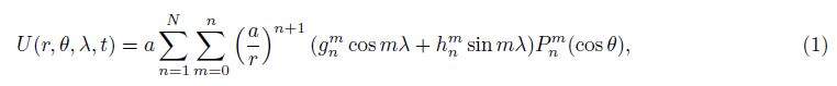
2 COMPUTING CRUSTAL MAGNETIC FIELDAccording to the theory of geomagnetic field potential function, geomagnetic potential can be expressed as spherical harmonic series:
According to the rule of geomagnetic field energy spectrum varying with harmonic order, it is normally believed that spherical harmonic order n ≤ 13 is ascribed to core field, n = 14 ~ 15 is ascribed to the transition between core and crustal magnetic fields, and n ≥ 16 is primarily ascribed to crustal magnetic field[23]. In POMME-6.2 model, the maximum truncation order N = 740, as 721~740-order model coefficients are almost zero, this paper takes truncation order N = 720 for computing. To calculate total intensity of crustal magnetic field △F, one has to calculate the intensity values of total magnetic field of order n = 1 ~ 720 and that of core magnetic field of order n = 1 ~ 15 respectively, then subtract core field intensity from total magnetic field intensity, and the difference will be the intensity of crustal magnetic field △F. Taking the derivative of total geomagnetic field intensity with respect to geocentric distance r[24] yields the vertical gradient of crustal magnetic field ∂(△F)/∂r. Setting r ≥ a, we can calculate crustal magnetic anomaly distribution over the ground and at various altitudes above ground (h).
Since the influences of Eastern Syntaxis on the crustal magnetic anomalies of the surrounding area is striking, this paper selects a study area of 22°N-34°N and 87°E-108°E with grid spacing being 0.1°×0.1°. The area geographically involves the central Tibetan Plateau, Eastern Syntaxis region, Sichuan-Yunnan region, North India and Northwest Myanmar region. Fig.2 presents the anomaly distribution of ground-based (h =0km) crustal magnetic field △F and its vertical gradient ∂(△F)/∂r, and the anomaly distribution of crustal magnetic field at altitudes above ground (h = 25 km and h = 100 km respectively). The red-line boxes in ∂(△F)/∂r anomaly distribution map (from left to right) are the central Tibetan Plateau, Eastern Syntaxis and Central Yunnan region respectively. Because strong anomalies only appear in local areas, we choose a color for area with anomaly greater than a certain value, in order to clearly show the weak anomaly in the plateau. For example, anomaly of △F > 120 nT was selected as one kind of color.

|
Fig.2 Distribution of the crustal magnetic anomaly at different altitudes |
As shown in Fig.2a, the distribution of the crustal magnetic anomaly on the ground surface in the study region has obvious regional characteristics. The positive magnetic anomalies over Sichuan Basin are large in area and high in intensity. In Himalayan Orogenic Belt, and the region of Longmen Mountains and Daba Mountains on the north of Sichuan Basin, there are approximately east-west strong negative magnetic anomaly belts. In the central Tibetan Plateau on the northwest of Eastern Syntaxis, there are positive and negative magnetic anomaly bands in approximately east-west strike. In Central Yunnan massif, positive and negative magnetic anomalies are lumpy and banded. Elsewhere, magnetic anomalies are relatively weak, but under the setting of weak magnetic anomaly, positive and negative magnetic anomalies in northeast direction over Eastern Syntaxis exhibit arc-shaped distribution. The outermost arc-shaped magnetic anomaly belt runs roughly along Jinshajiang-Honghe Fault Belt, basically consistent with the fault strike.
The ground magnetic anomaly △F basically agreed with the anomaly of vertical gradient ∂(△F)/∂r (Fig.2b) in terms of distribution shape and strike, but the scopes of strong and weak anomalies differed dramatically. The vertical gradient values are not only related with rock magnetism but also immediately associated with both distribution and depths of magnetic-source bodies. The deeper and more uniformly distributed the magnetic-source bodies, the smaller the vertical gradients are. Conversely, when magnetic-source bodies are shallow and non-uniformly distributed, the vertical gradient values change much. The ground magnetic anomalies (△F) over positive anomaly zone in Sichuan Basin and negative anomaly zones including Himalaya and Longmen Mountains spread widely with high intensity, nevertheless, vertical gradients (∂(△F)/∂r) do not show any strong anomalies over respective regions. This reflects a relatively uniform spatial distribution of magneticsource bodies in such regions. In the central Tibetan Plateau and Central Yunnan massif, magnetic anomalies and vertical gradient anomalies are basically consistent in distribution shape, strike and anomaly focus, but positive and negative magnetic anomalies alternate and spread over a small scope, indicating that magnetic materials of both regions are shallowly buried and non-uniformly distributed. Along Jinshajiang-Honghe Fault Belt, the arc-shaped gradient anomaly belt was sharper.
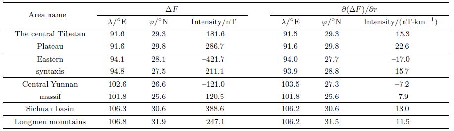
For a quantitative understanding of the characteristics of magnetic anomaly intensity, Table1 lists the foci and intensities of △F and ∂(△F)/∂r over the major ground anomaly zones. For Central Yunnan massif and the central Tibetan Plateau where there are numerous magnetic anomaly foci, Table1 shows only two points with the strongest positive and negative anomalies. From Table1, the magnetic anomalies are the strongest over Sichuan Basin and eastern Syntaxis region; the foci of magnetic anomalies do not coincide fully with those of gradient anomalies; magnetic anomaly intensity is not definitely proportional to vertical gradient. For example, the vertical gradient of the central Tibetan Plateau has the greatest positive anomaly focus value, but its magnetic anomaly focus value is far less than positive anomaly over Sichuan Basin. Table1 gives positions and intensities of major anomaly foci in various massifs, including: the central Tibetan Plateau, Eastern Syntaxis, Central Yunnan massif, Sichuan Basin, and Longmen Mountains.
| Table 1 The location and intensity of magnetic anomaly centers of △F and ∂(△F)/∂r for the blocks on earth’s surface |
Analyzing the distribution of magnetic anomaly at different altitudes above ground can help understand the depths of magnetic anomaly sources. By extrapolating ground magnetic anomaly upward, we calculated magnetic anomaly distribution at various altitudes above ground. Figs. 2c and 2d give magnetic anomaly distributions at 25 km and 100 km altitudes, respectively. It is observed from magnetic anomalies at different altitudes that, as the altitude increases, there are significant differences in magnetic anomaly decay among regions. In Sichuan Basin and Himalaya-Eastern Syntaxis-Longmen Mountains region, positive and negative magnetic anomalies decayed slowly. At 100 km altitude in Sichuan Basin, the positive anomaly exhibited oval distribution, agreeing with the basin’s configuration. Other regions exhibited negative anomalies, the strong negative magnetic anomaly belt remaining in Himalaya-Eastern Syntaxis-Longmen Mountains region joined the negative anomaly zone in Tibetan Plateau. In the central Tibetan Plateau and Central Yunnan massif, banded and lumpy magnetic anomalies decayed quickly, and almost disappeared completely at 25km altitude, indicating that they are shallow-seated local anomalies superposed onto negative anomaly setting.
3.3 Two-Dimensional Wavelet Decomposition of Magnetic AnomaliesThe changes of the magnetic anomalies with altitude in section 3.2 indicate that the decay of magnetic anomaly varies greatly with region, and that magnetic anomaly field is a superposition result of anomalies arising from subsurface magnetic-source bodies with various depths, scales and shapes. The wavelet transform method developed in recent years is able to decompose a potential field into components of various scales, and has been well applied in gravity field, aeromagnetic anomaly, etc.[25, 26]. Since local magnetic anomalies are shallowly buried, whereas regional fields are deeply buried, they have different wavelet transform decay rates on different scales. Hence, choosing appropriate decomposition scale can probably distinguish them from each other.
3.3.1 Characteristics of two-dimensional wavelet decomposition of magnetic anomaliesAccording to two-dimensional wavelet transform principle[27, 28], a potential field can be decomposed into detail signal Dn[f(x, y)] and approximation signal (smooth approximation) An[f(x, y)]on various spatial scales, the anomaly signal after N-order wavelet decomposition can be expressed as
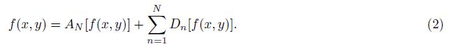
The key to wavelet decomposition of crustal magnetic anomalies is to choose an appropriate wavelet function. After comparing several wavelet functions through trial calculation, we employed relatively orthogonal Daubechies (db5) wavelet function to decompose the ground magnetic anomalies[29, 30, 31]. According to low-order wavelet detail invariability principle[32], we firstly observed distribution characteristics of various orders of details and approximation signal during magnetic anomaly wavelet decomposition, and then chose appropriate decomposition scales and their combinations. Results of decomposing the ground magnetic anomalies show that, 1~3 orders of wavelet details have small spatial scales with similar distribution shapes, and 4~5 orders of wavelet details have larger spatial scales with similar anomaly distribution features. Consequently, we chose wavelet truncation order to be 5 and combined 1~3 orders and 4~5 orders of wavelet details respectively.
Figs. 3a, 3b and 3c give anomaly distribution maps of the ground magnetic anomalies, including combination of 1~3 orders of wavelet details (D1 + D2 + D3), combination of 4~5 orders of wavelet details (D4 + D5), and 5-order wavelet approximation (A5).

|
Fig.3 The magnetic anomaly distribution for wavelet (left) and different wavelength bands (right) |
Figure3a shows that the anomalies with combination of 1~3 orders of wavelet details have smaller spatial scales, and are primarily banded and lumpy. The anomaly in central Tibetan Plateau is in east-west strike, while that in Longmenshan massif is in north-east strike. In the combination of 4~5 orders of details (Fig.3b), there is positive anomaly over Sichuan Basin, with negative anomaly belts in the south and north of it. On the north of Himalaya strong negative anomaly belt, there is a parallel positive anomaly belt, which extends all the way to the dome of Eastern Syntaxis region and envelops Himalaya negative anomaly belt. In north-east direction of the eastern Syntaxis dome, there are alternating positive and negative arc-shaped weak anomaly belts. Regional anomalies reflected by 5-order approximation signal (Fig.3c) have simple distribution shapes, with positive anomaly over Sichuan Basin and negative anomaly belt or weak anomaly elsewhere. The arc-shaped anomaly in north-east direction of Eastern Syntaxis shown in wavelet details totally disappears in 5-order approximation.
3.3.2 Equivalent depths of magnetic anomaly sourcesWavelet transform is a kind of mathematical tool that can decompose a magnetic anomaly into components of various scales, but cannot give geophysical implications of various scales of components. To know geophysical implication of anomaly distribution derived from wavelet decomposition, we used the radial power spectrum analysis to determine the depths of magnetic sources corresponding to wavelet combination anomalies. We also compared magnetic anomalies with wavelet detail combinations against those over various wavelength belts. According to the theory of potential field wavenumber domain, the increment of power spectrum slope is directly proportional to that of field source depth. Therefore, wavelet details and depths of magnetic field sources corresponding to approximation can be calculated from power spectrum slope, so that wavelet analysis results have corresponding depth concepts. From perspective of statistics, the fitting straight lines for radial mean power spectra of magnetic anomalies reflect equivalent depths of anomaly field sources[33, 34].
Non-uniform magnetic anomaly intensities and distribution over the study area imply that magnetic anomaly source varies in scale and depth. According to distribution characteristics of wavelet detail combined magnetic anomalies, we firstly divided the study area into three sections, namely, the central Tibetan Plateau (26°N-34°N, 87°E-97°E), Sichuan Basin-Longmen Mountains (28°N-34°N, 98°E-108°E), and Central Yunnan (22°N-28°N, 98°E-108°E). And then we employed radial power spectrum method to calculate equivalent depths of magnetic anomaly bodies in various sections respectively (Fig.4)[35, 36]. Symbols a, b, and c in Fig.4 represent the central Tibetan Plateau, Sichuan Basin-Longmen Mountains, and Central Yunnan sections, respectively. For all sections, equivalent depths of 1~3 orders of wavelet detail combination range from 9 km to 12 km, and that of 4~5 orders of wavelet detail combination range from 26 km to 29 km. In respect of linear fitting effect of power spectra, 4~5 orders of detail combination is better than 1~3 orders of detail combination, indicating that non-uniform spatial distribution of the upper crust magnetic-source bodies is more intense. As to central Yunnan section, the equivalent depths of 1~3 orders of wavelet detail combined anomalies are shallower (9 km), but those of 4~5 orders of detail combined anomalies are deeper (29 km).

|
Fig.4 The power spectra of the wavelet details reconstruction |
Equivalent depths of magnetic-source bodies given by wavelet detail combination basically agreed with the crustal stratification revealed by seismology. Zhang et al. employed seismic surface wave dispersion to rebuild S-wave velocities in the crust and mantle of Sichuan-Yunnan region[37], and found that the crust of Yunnan region consists of the upper and the lower layers, where the thickness of the upper crust does not vary much, mostly ranging from 10 km to 15 km. Peng et al. employed receiver function and magnetotelluric data to conduct joint inversion of crust-mantle structures of Eastern Himalayan Syntaxis region[38], and demonstrated that crust-mantle structures of the central eastern Syntaxis consist of the upper, middle and lower layers. The upper crust has high resistance and high velocity layers of 9~14 km thick. On the other hand, the average depth to middle crust is 28 km. As can be seen, average equivalent depth of 1~3 orders of wavelet detail combined magnetic-source bodies basically agrees with that of 4~5 orders of combination.
3.3.3 Correspondences between magnetic anomalies over various wavelength belts and wavelet decompositionAs calculated, spherical harmonic orders of crustal magnetic anomalies range in 16~720, and the corresponding spatial wavelengths approximately fall within 2500~56 km[23]. According to changes in crustal magnetic field energy spectra[10], crustal magnetic fields can be divided into long-wavelength belt (16~60 orders), medium-wavelength belt (61~220 orders) and short-wavelength belt (221~720 orders). Figs. 3d, 3e and 3f give magnetic anomaly distribution of three kinds of wavelength belts respectively. Comparison between magnetic anomalies over various wavelength belts and those from wavelet decomposition reveals an excellent correspondence between the detail combination of 1~3 order wavelets and the short-wavelength belt, between the detail combination of 4~5 order wavelets and the medium-wavelength belt, and between the 5-order approximation and the long-wavelength belt. This indicates that the wavelet decomposed magnetic anomalies are specific reflection of magnetic anomalies over various spatial wavelengths.
3.4 Relationship Between Magnetic Anomaly and Geological StructureThe above analysis indicates that, the crustal magnetic anomalies over the study area except Sichuan Basin are medium- and short-wavelength anomalies superposed onto negative or weak magnetic anomaly setting, and such magnetic anomalies are very well associated with the geological structures.
Studies on the geology, geomorphology and geophysical field in the northwest of the eastern Syntaxis indicate that the giant east-west structures are the most obvious tectonic feature[7, 39]. In the north of Himalayan Orogenic Belt, the east-west magnetic anomaly bands are relatively strong, consistent with tectonic strike of the plateau. In particular, the east-west magnetic anomaly bands within 28°N-32°N and 87°E-94°E are especially conspicuous.
In eastern Syntaxis, Indian Plate pushes northward against Tibetan Plateau with a velocity of 47 mm/a (approx. NE 23°)[40], and the northeastern corner of Indian Plate, resembling a wedge, plunges in the northeast direction into the southeastern margin of the plateau, causing an important impact on the surrounding regions. Studies such as GPS horizontal displacement[41, 42], seismic wave velocity structure[43, 44], magnetotelluric survey[45] show that, massifs on the north and east of Eastern Syntaxis generally turn clockwise around the tectonic syntaxis, resulting in an arc-shaped structure. In north-east direction of eastern Syntaxis, both magnetic anomaly after wavelet detail combination and magnetic anomaly over medium- and short-wavelength belts (Fig.3) exhibited positive and negative alternating arc-shaped distribution, reflecting the arc-shaped tectonic feature of the middle and upper crust magnetic-source bodies.
In Northwest Sichuan, west Yunnan and Sanjiang orogenic belts, which lie on the east of eastern Syntaxis and the west of Longmen Mountains-Xiaojinhe-Honghe Fault Belt, the crustal magnetic anomalies are weak. Magnetic anomaly values are small in the scope of approximately 98°E-101°E, which constitute the approximately south-north direction weak magnetic anomaly belt. This is the central and southern part of China’s south-north seismic belt, and the youngest orogenic belt, too.
Since the approximately south-north underthrusting Indian Plate collided with Eurasian Continent and the Tibetan Plateau is blocked by Siberian platform in the north, the crustal material flowed eastward, and then, blocked by a high-intensity massif (Sichuan Basin), it forked into east-north and east-south strikes. In Longmen Mountains region on the north of Sichuan Basin, as for the vertical gradient anomaly reflecting the anomalies of the middle and upper crust magnetic-source bodies (Fig.2), 1~3 orders of wavelet detail combination and shortwavelength belt have distinct north-east strike, consistent with that of geological structures. Bai et al. studied the lower crustal flow in the southeastern part of Tibetan Plateau by means of magnetotelluric tomographic imaging, and further gave the position of the lower crustal flow[45]. In the east of Tibetan Plateau, there exist two giant low-resistivity anomaly belts in the middle and lower crust, one extends eastward from Lhasa massif along Yarlung Zangbo suture zone, circumvents eastern Himalayan syntaxis and turns southward; the other extends eastward from Qiangtang terrane along Jinshajiang-Xianshuihe Fault Belt, turns southward in the western margin of Sichuan Basin, and finally passes through lozenge-shaped Sichuan-Yunnan massif (Central Yunnan massif) between Xiaojiang Fault and Honghe Fault. In Central Yunnan massif, positive and negative magnetic anomalies are relatively strong, appearing banded and lumpy. The rule of their decaying with altitude is the same as that of banded anomalies over the central Tibetan Plateau. This indicates that the magnetic-source bodies of Central Yunnan massif are part of Tibetan Plateau crustal material flowing southeastward.
Comparison between magnetic anomaly distribution and fault belt distribution shows that, Longmenshan Fault Belt, Lijiang-Xiaojinhe Fault Belt and Honghe Fault Belt are distinct boundaries between strong and weak magnetic anomalies. Whereas, intensities of crustal magnetic anomalies over both sides of Xianshuihe Fault Belt, Nujiang Fault, and Lancangjiang Fault Belt have no significant difference, indicating that magnetic material distribution does not change much over both sides of such faults.
4 CONCLUSIONS(1) The ground magnetic anomalies around eastern Syntaxis given by POMME6.2 model have distinct regional characteristics. Sichuan Basin and eastern Syntaxis have strong positive magnetic anomalies, whereas Himalaya and Longmenshan massifs have strong negative magnetic anomalies. Over the central Tibetan Plateau and Central Yunnan massif, the magnetic anomalies are relatively strong, exhibiting banded and lumpy distribution. Elsewhere, magnetic anomalies are weaker.
(2) Crustal magnetic anomalies around eastern Syntaxis are closely associated with geological structures. Analyses of magnetic anomaly distribution at various altitudes and over various wavelength belts, wavelet decomposed detail combined anomalies, and approximation anomalies indicate that, all magnetic anomalies around eastern Syntaxis (except Sichuan Basin) are medium- and short-wavelength positive and negative magnetic anomalies superposed onto negative or weak magnetic anomaly setting. These meso- and micro-scale magnetic anomalies arise from magnetic materials in the middle and upper crust, with the same strike as geological structures. Longmenshan Fault Belt, Lijiang-Xiaojinhe Fault Belt and Honghe Fault Belt are the boundary between positive and negative magnetic anomalies, or the transitional zone between strong and weak anomalies.
(3) Eastern Syntaxis has important impact on crustal magnetic anomalies over its surrounding area. The east-west magnetic anomaly bands in the central Tibetan Plateau exhibit arc-shaped distribution over the dome of Eastern Syntaxis, consistent with tectonic shape given by geological field and relevant geophysical field. The positive magnetic anomalies over eastern Syntaxis region primarily arise from the middle and upper crust. Various distribution morphological features of crustal magnetic anomalies around eastern Syntaxis given in this paper provide crustal magnetic anomaly evidence for geological and geophysical researches on the collision between Indian Plate and Eurasian Plate, as well as the Tibetan Plateau uplift and their material transport.
ACKNOWLEDGMENTSThis work was supported by the National Natural Science Foundation of China (41264003) and Key Projects of Natural Science Foundation of Provincial Education Department of Yunnan (2012Z048).
| [1] Schoenbohm L M, Burchfiel B C, Chen L Z. Propagation of surface uplift, lower crustal flow, and Cenozoic tectonics of the southeast margin of the Tibetan Plateau. Geology, 2006, 34(10): 813-816. |
| [2] Wang E Q, Barchfiel B C, Ji J Q. Estimation of Cenozoic crust shortening and its geological evidence in Himalayas structure knot. Science in China (Seies D) (in Chinese), 2001, 31(1): 1-9. |
| [3] Song J, Tang F T, Deng Z H, et al. Study on current movement characteristics and numerical simulation of the main faults around Eastern Himalayan Syntaxis. Chinese J. Geophys. (in Chinese), 2011, 54(6): 1536-1548. |
| [4] Teng J W, Wang Q S, Wang G J, et al. Specific gravity field and deep crustal structure of the "Himalayas east structural knot". Chinese J. Geophys. (in Chinese), 2006, 49(4): 1045-1052. |
| [5] An Z C. Studies on geomagnetic field models of Qinghai-Xizang plateau. Chinese J. Geophys. (in Chinese), 2000, 43(3): 339-345. |
| [6] He R Z, Gao R, Zheng H W, et al. Matched-filter analysis of aeromagnetic anomaly in mid-western Tibetan Plateau and its tectonic implications. Chinese J. Geophys. (in Chinese), 2007, 50(4): 1131-1140. |
| [7] Xue D J, Jiang M, Wu L S, et al. East-west division of regional gravity and magnetic anomalies on the Qinghai-Tibet plateau and its tectonic features. Geology of China (in Chinese), 2006, 33(4): 912-919. |
| [8] Xiong S Q, Zhou F H, Yao Z X, et al. Aero magnetic survey in central and western Qinghai Tibet Plateau. Geophysics & Geochemical Exploration (in Chinese), 2007, 31(5): 404-407. |
| [9] Zhang C D. The magnetic characteristics of crust beneath Xizang (Tibetan) plateau deduced from satellite magnetic anomaly. Progress in Geophysics (in Chinese), 2002, 17(2): 325-330. |
| [10] Kang G F, Gao G M, Bai C H, et al. Characteristics of the crustal magnetic anomaly and regional tectonics in the Qinghai-Tibet Plateau and the adjacent areas. Sci. China-Earth Sci., 2012, 55(6): 1028-1036. |
| [11] Xu W Y, Bai C H, Kang G F. Global models of the Earth's crust magnetic anomalies. Progress in Geophysics (in Chinese), 2008, 23(3): 641-651. |
| [12] Hemant K, Thbault E, Mandea M, et al. Magnetic anomaly map of the world: merging satellite, airborne, marine and ground-based magnetic data sets. Earth Planet Sci. Lett., 2007, 260(1-2): 56-71. |
| [13] Olsen N, Lühr H, Sabaka T J, et al. CHAOS-a model of the Earth's magnetic field derived from CHAMP, ørsted and SAC-C magnetic satellite data. Geophys. J. Int., 2006, 166(1): 67-75. |
| [14] Olsen N, Mandea M, Sabaka J T, et al. CHAOS-2 a geomagnetic field model derived from one decade of continuous satellite data. Geophys. J. Int., 2009, 179(3): 1477-1487. |
| [15] Sabaka T J, Olsen N, Purucker M E. Extending comprehensive models of the Earth's magnetic field with ørsted and CHAMP data. Geophys. J. Int., 2004, 159(2): 521-547. |
| [16] Hamoudi M, Thébault E, Lesur V, et al. Geoforschungs Zentrum anomaly magnetic map (GAMMA): A candidate model for the world digital magnetic anomaly map. Geochem. Geophys. Geosyst., 2007, 8(6), doi: 10.1029/2007 GC001638. |
| [17] Maus S, Rother M, Stolle C, et al. Third generation of the Potsdam magnetic model of the Earth (POMME). Geochem. Geophys. Geosyst., 2006, 7(7), doi: 10.1029/2006GC001269. |
| [18] Maus S. An ellipsoidal harmonic representation of Earth's lithospheric magnetic field to degree and order 720. Geochem. Geophys. Geosyst., 2010, 11, Q06015, doi: 10.1029/2010GC003026. |
| [19] Maus S, Lühr H, Rother M, et al. Fifth-generation lithospheric magnetic field model from CHAMP satellite measurements. Geochem. Geophys. Geosyst., 2007, 8(5), doi: 10.1029/2006GC001521. |
| [20] Maus S, Barckhausen U, Berkenbosch H, et al. EMAG2: A 2-arc min resolution Earth Magnetic Anomaly Grid compiled from satellite, airborne, and marine magnetic measurements. Geochem. Geophys. Geosyst., 2009, 10(8), Q08005, doi: 10.1029/2009GC002471. |
| [21] Maus S, Manoj C, Rauberg J, et al. NOAA/NGDC candidate models for the 11th generation international geomagnetic reference field and the concurrent release of the 6th generation Pomme magnetic model. Earth, Planets and Space, 2010, 62(10): 729-735. |
| [22] Xu W Y. Physics of Electromagnetic Phenomena of the Earth (in Chinese). Hefei: University of Science and Technology of China Press, 2009: 93-101. |
| [23] Thébault E, Purucker M, Kathryn A, et al. The Magnetic Field of the Earth's Lithosphere. Space Sci. Rev., 2010, 155(1-4): 95-127. |
| [24] Gao G M, Kang G F, Bai C H, et al. Characteristics of the spatial distribution and the secular variation of the main geomagnetic field gradients. Chinese J. Geophys. (in Chinese), 2012, 55(8): 2651-2659. |
| [25] Hornby P, Boschetti F, Horowitz H G. Analysis of potential field data in the wavelet domain. Geophys. J. Int., 1999, 137(1): 175-196. |
| [26] Wu Y, Meng X H, Li S L. Wavelet analysis and its application in geophysics of China. Progress in Geophysics (in Chinese), 2012, 27(2): 750-760. |
| [27] Hou Z Z, Yang W C. Wavelet transform and multi-scale analysis on gravity anomalies of China. Chinese J. Geophys. (in Chinese), 1997, 40(1): 85-95. |
| [28] Chambodut A, Panet I, Mandea M, et al. Wavelet frames an alternative to spherical harmonic representation of potential fields. Geophys. J. Int., 2005, 163(3): 875-899. |
| [29] Daubechies I. The wavelet transform, time-frequency localization and signal analysis. IEEE Transactions on Information Theory, 1990, 36(5): 961-1006. |
| [30] Daubechies I, Sweldens W. Factoring wavelet transforms into lifting steps. J. Fourier Anal. Appl., 1998, 4(3): 247-269. |
| [31] Marlet G, Sailhac F, Moreau F, et al. Characterization of geological boundaries using 1-D wavelet transform on gravity data: Theory and application to the Himalayas. Geophysics, 2001, 66(4): 1116-1129. |
| [32] Hou Z Z, Yang W C. Multi-scale inversion of density structure from gravity anomalies in Tarim Basin. Science in China (Seies D), 2011, 54(3): 399-409. |
| [33] Bhattacharyya B K, Leu L K. Spectral analysis of gravity and magnetic anomalies due to two-dimensional structures. Geophysics, 1975, 40(6): 993-1013. |
| [34] Spector A, Grant F S. Statistical models for interpreting aeromagnetic data. Geophysics, 1970, 35(2): 293-302. |
| [35] Zhang X, Zhao L. An analysis of the power spectrum for computing field source depths of magnetic bodies of different scales. Geophysical & Geochemical Exploration (in Chinese), 2007, 31(Suppl.): 53-56. |
| [36] Vallée M A, Keating R S, Smith R S, et al. Estimating depth and model type using the continuous wavelet transform of magnetic data. Geophysics, 2004, 69(1): 191-199. |
| [37] Zhang Z, Chen Y, Li F. Reconstruction of the S-wave velocity structure of crust and mantle from seismic surface wave dispersion in Sichuan-Yunnan region. Chinese J. Geophys. (in Chinese), 2008, 51(4): 1114-1122. |
| [38] Peng M, Tan H D, Jiang M, et al. Joint inversion of receiver functions and magnetotelluric data: Application to crustal and mantle structure beneath central Namche Barwa, eastern Himalayan syntaxis. Chinese J. Geophys. (in Chinese), 2012, 55(7): 2281-2291. |
| [39] Zhang J, Ma Z J. East-West segmentation of the Tibetan plateau and its implication. Acta Geologica Sinica (in Chinese), 2004, 78(2): 218-227. |
| [40] Paul J, Bürgmann R, Gaur V K, et al. The motion and active deformation of India. Geophysical Research Letters, 2001, 28(4): 647-650. |
| [41] Cao J L, Shi Y L, Zhang H, et al. Numerical simulation of GPS observed clockwise rotation around the eastern Himalayan syntax in the Tibetan Plateau. Chinese Science Bulletin, 2009, 54(8): 1398-1410. |
| [42] Wang Q, Zhang P Z, Freymueller J T, et al. Present-day crustal deformation in China constrained by global positioning system measurements. Science, 2001, 294(5542): 574-577. |
| [43] Cui Z X, Pei S P. Study on Pn velocity and anisotropy in the upper most mantle of the Eastern Himalayan syntaxis and surrounding regions. Chinese J. Geophys. (in Chinese), 2009, 52(9): 2245-2254. |
| [44] Wang C Y, Han W B, Wu J P, et al. Crustal structure beneath the eastern margin of the Tibetan plateau and its tectonic implications. J. Geophys. Res., 2007, 112: B07307, doi: 10.1029/2005JB003873. |
| [45] Bai D H, Unsworth M J, Meju M A, et al. Crustal deformation of the eastern Tibetan plateau revealed by magnetotelluric imaging. Nature Geoscience, 2010, 3(5): 358-362. |