 2013, Vol. 56


The term full-waveform inversion (FWI) was first proposed by Pan et al. (1986),although the method was described in the early 1980’s. Its framework was based on the data-fitting principle described by Tarantola (1987). The gradient of the objective function in traditional FWI was calculated by the adjoint-state method[1, 2, 3, 4]. Great improvements have been made in the last ten years. FWI has been applied to the study of global or regional crust and upper mantle structure[5] and has been found to provide more accurate background velocity models for imaging in oil and gas exploration[6]. FWI has great potential for quantitative reservoir monitoring[7, 8],lithology and fluid identification,and crack characterization research[9]. It provides subsurface images with higher resolution for geodynamics research and seismic exploration.
The goal of FWI is to find a subsurface model by minimizing the residual between the synthetic data and the observed data. Theoretically,FWI can provide a model with much higher resolution than conventional methods,but it has not been widely used so far. In seismology,it cannot yet replace traditional travel-time tomography and finite-frequency tomography. In seismic exploration,it has not taken the place of the conventional workflow of seismic data processing and interpretation. In addition to certain practical problems such as low signal-tonoise ratio,lack of low frequencies,unknown source wavelets,and the difficulty of describing accurately seismic wave propagation in complex media,strong nonlinearity has been the biggest problem in both theory and application of FWI.
The strong nonlinearity of FWI originates from the complexity of seismic wave propagation in the subsurface. Therefore,parameter estimation from received seismic data becomes a very complex process. At present,this difficult problem is usually solved using a multi-step procedure. The background of the velocity model (the low-wavenumber variations in velocity) is obtained through NMO velocity analysis,migration velocity analysis (MVA),or travel-time tomography. The reflectivity of the subsurface structure (the high-wavenumber variations in velocity) is resolved by seismic imaging (stacking or migration). Then the rock physics properties are inverted by amplitude versus offset (AVO) inversion,impedance inversion,or seismic attribute analysis on the basis of relative amplitude-preserving data processing. One advantage of this conventional seismic imaging and inversion workflow is that manual intervention can be used during the process,although it requires substantial time and labor resources.
To overcome the strong nonlinearity in seismic inversion,FWI should not be a “black box”. Rather,inversion should be accomplished in a multi-step and multi-scale way. This is the inversion strategy used in FWI.
The essence of this strategy is how to solve a complex inversion problem in a multi-stage and multi-scale way. The goal is to construct a new objective function with lower nonlinearity using a different seismic data subset in each inversion stage to improve the convergence and inverse resolution of FWI.
Many factors can cause strong nonlinearity in FWI,and therefore a single inversion strategy often appears to be too limiting. Besides some practical problems,such as low signal-to-noise ratio,limited observation apertures,and unknown source wavelets,the main reason for strong nonlinearity is the complexity of the relationship between the seismic data and the subsurface parameters. Technically speaking,it represents the strong nonlinearity of the objective function. The choice of objective function is related to many technical problems. The stronger the nonlinearity of the objective function,the more accurate must be the starting model and the more sophisticated the inversion strategy. Therefore,the objective function plays a crucial role in FWI. It embodies how the seismic data change with parameter perturbations,which is called the sensitivity kernel. This is one of the most important problems in seismology. The relationship between perturbation of the seismic data under different kinds of objective function and perturbation of physical parameters is of great importance in seismic inversion. It directly determines whether the objective function is appropriate,whether the inversion method is reasonable,whether the starting model meets requirements,and consequently what kinds of inversion strategy should be chosen. Therefore,analysis of the behavior of objective functions calculated from different seismic data subsets and their variation with the scale of parameter perturbations is the basis of multi-step and multi-scale FWI. Although it is impractical to attain a comprehensive understanding of objective-function variation by arbitrary perturbations of model parameters,we can analyze the behavior of the objective function in certain ways. In particular,we can investigate the behavior of the objective function and its variations with the scale of parameter perturbations.
On this topic,Claerbout[10] found that reflected seismic data did not contain ultra-short wavelength information on the medium. Snieder et al.[11] discussed the possibility of decoupling short- and long-wavelength velocity components. Liu and Dong[12] investigated possibilities for inversion using seismic reflection data and numerical experiments. Hicks and Pratt[13] suggested a two-step inversion procedure for both high- and lowwavenumber velocity components based on analysis of the relationship between seismic data perturbations and physical parameters. Wang and Rao[9] and some other authors have suggested that the long-wavelength velocity component should be obtained by travel-time tomography,while the short-wavelength component should be resolved by waveform inversion.
Jannane et al.[14] made outstanding contributions in this respect. They investigated the variation of an objective function with velocity and impedance perturbations (see Fig.1) through numerical simulation of seismic wave propagation in which the L2 norm of the seismic reflection residual data was used as an objective function. They concluded that the seismic reflection travel time was sensitive to the long-wavelength velocity components,while the amplitude was sensitive to the short-wavelength components,and that it was hard to resolve medium-wavelength components using seismic reflection data (see also Sears et al.[15]). This literature has been cited by many authors because it plays an important role in choosing appropriate inversion methods and strategies. The Society of Exploration Geophysicists (SEG) international annual meeting in 2010 held a special workshop on this article for its outstanding contribution[16].

|
Fig.1 Dependence of the misfit functions on the perturbation scale of velocity and impedance[14] |
However,because of insufficient computational capability at that time,there were several disadvantages in the method proposed by Jannane et al.[14]. First of all,they only discussed objective functions based on the L2 norm,whereas several kinds of objective functions are being used in FWI at present. Second,they analyzed only variations in P-wave velocity,density,and impedance,which meant that their conclusions could not be extended to more general models involving anisotropy or attenuation. Third,they investigated only vertical variations in spatial wavelength,although 3D parameter variations were needed in FWI. Fourth,they calculated the objective function using the entire set of seismic data,without analyzing the behavior of objective function using subsets of seismic data. This affected the choice of an appropriate inversion strategy. In fact,choosing different subsets of seismic data is an effective approach to reduce the strong nonlinearity of seismic inversion using a multi-step and multi-scale strategy. By analyzing the behavior of objective functions calculated using different seismic data subsets,it is possible to provide theoretical guidance for the choice of reasonable seismic data subsets and specific inversion strategies in different inversion stages. These data subsets include specific arrivals (first arrivals,reflections,and refractions),specific information (travel-time,amplitude,phase,and frequency),specific apertures (different offsets and time windows),and so on. Finally,the maximum offset was 1760 m in their numerical experiments,however,the maximum offset in modern onshore or offshore data acquisition is usually greater than 10 km. Because different behavior was observed for objective functions calculated using seismic data with different offsets,the conclusions obtained with such limited maximum offset data are inevitably one-sided.
The disadvantages described above meant that the conclusions obtained by Jannane et al. (1989) had certain limitations for practical use in FWI. These limitations not only affected the choice of specific inversion strategies,but also were unfavorable to choosing an appropriate objective function. Therefore,whether from the viewpoint of understanding wave propagation in depth,or from the viewpoint of improving the theoretical foundations of FWI,optimizing the choice of inversion strategy,constructing better objective functions,and choosing an appropriate model parameterization,further detailed study on this problem is required. Furthermore,research into this problem will also be very helpful to development of other seismic inversion theories and methods (e.g.,travel-time tomography,AVO inversion) and their practical use.
In this research,we have investigated the relationship between objective functions calculated using different seismic data subsets and the scale of perturbation of the model parameters (such as velocity,density,impedance,and bulk modulus). The behavior of various objective functions has been analyzed using high-precision numerical simulation of wave propagation in variable-density acoustic media with the intent of overcoming the limitations of Jannane et al.[14] and providing theoretical guidance for the choice of an objective function,the construction of the covariance matrix,and the formulation of an inversion strategy.
2 EXPERIMENTAL METHODS 2.1 Reference ModelA sonic log from a marine well was chosen as the reference model. The depth of the model was 2075 m, and its density ρ0(z) and velocity V0(z) curves are shown in Fig.2.

|
Fig.2 Density and velocity curves of the reference model |
To analyze the behavior of the objective function,sinusoidal perturbations were imposed at different wavelengths λ on the media parameters. For instance,the density perturbation with depth was calculated as ρ(z) = ρ0(z)+△ρ(z) = ρ0(z)+0.10ρmax sin$(\frac{{2\pi }}{\lambda }z)$ ,where the perturbation quantity △ρ is a sinusoidal function of depth z,λ is the wavelength of the perturbation scale,and ρmax is the maximum value of the density model. The perturbation amplitude was ten percent of the maximum density. Fig.3 shows density perturbation curves at three scales (λ of 50 m,150 m,and 500 m).

|
Fig.3 Typical density perturbations at three scales (a) λ=50 m; (b) λ=150 m; (c) λ=500 m. |
To investigate the behavior of objective functions with different parameter perturbations,experiments were carried out for 11 specific parameter perturbations,as listed in Table1. Here,perturbations of velocity V and density ρ were considered,as well as of impedance I and bulk modulus K. Not only single perturbations were considered,but also simultaneous perturbations of two parameters were investigated.
| Table 1 Perturbation schemes of model parameters |
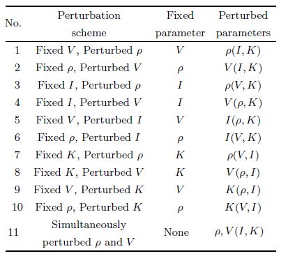
No additional perturbation models are shown here. Note that perturbation of one parameter (such as density) when the other (such as velocity) is fixed will cause the perturbation of other parameter classes (for example,impedance and bulk modulus).
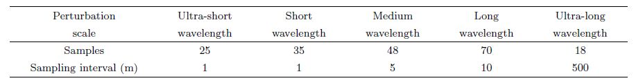
The different ranges of perturbation scale were defined as: the ultra-short wavelength band 0 m≤ λ ≤25 m,the short-wavelength band 25 m≤ λ ≤60 m,the medium-wavelength band 60 m≤ λ ≤300 m,the long wavelength band 300 m≤ λ ≤1000 m,and the ultra-long wavelength band λ ≥ 1000 m[14]. To represent the behavior of objective functions varying over entire scale bands,sample points were chosen densely at small scales,while sampling was sparse at large scales. There were 196 samples overall,as shown in Table2.
2.3 Objective FunctionIn seismic full-waveform inversion,different misfit functions,which measure the degree of matching between observed and simulated data,are selected for different inversion purposes. In this paper,three typical objective functions are analyzed: (1) L1and L2 norm objective functions for seismic data with different apertures; (2) L1 and L2 norm objective functions based on seismic trace envelopes,which can be obtained by Hilbert transforms; and (3) L1 and L2 norm objective functions constructed by Laplace transforms of seismic data.
| Table 2 Sampling distribution of the parameter perturbation scale |
A high-order finite-difference (FD) method was used to simulate seismic wave propagation[17]. The maximum offset was 9600 m,the trace interval was 10 m,961 traces were recorded for each shot,the sample interval was 1 ms,the recording time was 7 s,and the wavelet main frequency was 30 Hz (except where specially marked).
3 BEHAVIOR OF THE OBJECTIVE FUNCTION AND INVERSION STRATEGYThrough the experimental procedures described above,the characteristics of two kinds of objective functions (L1 and L2 norm) and how they varied with parameter perturbations for all seismic data sets or subsets (such as data sorted by different offsets,data trace envelopes,or signals after Laplace transform) were analyzed.
3.1 Relationship Between the Objective Functions Constructed by All Offsets and DifferentParameter Perturbation Scales Figure4 shows the sensitivity curves of the objective functions (L1 and L2 norm) and how they varied with parameter perturbation scale for all offsets (0~9600 m). The trends of the two objective functions were basically consistent (Figs. 4a and 4b),and therefore mainly the L2 norm will be analyzed in what follows. The difference is that the L1 norm is suitable for data in which the noise is Laplace distributed. Inversion is more stable but less sensitive using the L1 norm as the misfit function. Although the L2 norm is suitable for data in which the noise is Gaussian distributed,the inversion results are more sensitive to large outliers[18].

|
Fig.4 Dependence of the misfit functions on the perturbation scale of different media parameters according to seismic data for offsets from 0 to 9600 m (a) L1 norm; (b) L2 norm. |
The eleven curves shown in Fig.4 can be roughly divided into two categories. The first category consists of those in which density is perturbed while velocity is fixed (red lines 1,5,and 9). The rest of the curves,in which velocity is perturbed,can be classified into the second category.
For the first category in which only density is perturbed,the objective functions and their variations with parameter perturbation scale are relatively simple. Only when the perturbation scale is small (the perturbation wavelength is less than 200 m) does this category take on a quasi-quadratic form. This indicates that the objective function is extremely sensitive to small-scale density perturbations. When the density perturbation wavelength is large (more than 200 m),the objective functions are close to zero. The essential reason for this is that density perturbations do not change seismic travel time. However,small-scale density perturbations will change the reflection amplitude and thereby affect the value of the objective function. Because of the linear relationship between reflection amplitude variations and density perturbations,objective function variations with small density perturbations take on a quasi-quadratic form. However,density perturbations at medium and large scales cannot change travel time and therefore have little effect on reflection amplitude. Therefore,large-scale density perturbations cannot be inverted using reflected data. This is the “null space” problem in inversion.
On the other hand,except that the L1 norm objective function has slightly better properties with small velocity perturbations,the behavior of L1 norm objective-function variations with medium and large velocity perturbations and of L2 norm variations at all velocity perturbation scales are both worse (especially the L2 norm). Although the values of the objective functions are relatively large,they vary dramatically at all velocity perturbation scales (especially medium and large scales). Hence,it is not reasonable to invert all velocity perturbation components using small- and large-offset data (0~9600 m) simultaneously. However,the experimental results reported by Jannane et al. (1989)[14] demonstrated that L2 norm objective-function variations with small velocity perturbations take on a quasi-quadratic form,but then they concluded that small velocity perturbation components can be well resolved. The following analysis will indicate that they came to this conclusion because only small-offset data (less than 1760 m) were used.
Note that the objective function has relatively high values in the medium wavelength range for the second category of velocity perturbations,despite the complexity of the changes. This indicates that the objective function has some sensitivity to medium-wavelength velocity perturbations,which appear as relatively higher nonlinearity. This is different from the conclusion in Jannane et al. (1989) that reflected data cannot distinguish the medium velocity perturbation component. This conclusion may have been reached because only small-offset data (less than 1760 m) were used.
Figure4 shows the comprehensive performance of all offset seismic data in objective functions. Actually,the reflections of different parameter perturbation scales on the reflected data for various apertures are not the same. Hence,it is essential to analyze the behavior of objective functions using seismic data with different offsets and different parameterizations to propose a reasonable inversion strategy.
3.2 Relationships Between Objective Functions Constructed for Different Offsets and DifferentParameter Perturbation Scales Figure5 shows the sensitivity of the misfit functions (L2 norm) to the perturbation scale of different parameters,using seismic data with offsets from 0 to 600 m. It can be seen that Fig.5 is apparently different from Fig.4b. This illustrates that there are great differences in sensitivity for different perturbation scales of different parameters using different offset data. Therefore,it is important to use seismic data with different offsets during different stages of FWI. The perturbation curves shown in Fig.5 can be divided into four categories.

|
Fig.5 Dependence of the misfit functions (L2 norm) on the perturbation scale of different parameters using seismic data with offsets from 0 to 600 m |
The first category contains those cases in which density is perturbed while velocity is fixed (red solid line 1). The experiments for impedance and modulus perturbation are similar as long as the velocity is fixed (red lines 5 and 9). These three lines do not match completely because the density perturbations caused by perturbing different parameters are different. This kind of curve is almost quadratic for small-scale density perturbations (perturbation wavelengths less than 60 m). This indicates that the misfit function is very sensitive to small-scale density perturbations. However,the misfit function offers no information on medium- and longwavelength (λ ≥ 60) density perturbations. It can therefore be stated that medium- and long-wavelength density perturbations have almost no effect on reflected seismic data. Therefore,seismic reflection data with offsets less than 600 m cannot be used to invert medium- and long-wavelength density perturbations. This is because density perturbations have no influence on the travel time of seismic data,but small-scale density perturbations can change the reflection amplitudes (Fig.6a) and thereby affect the objective functions. However,the reflection data show no changes with medium- and long-wavelength density perturbations; neither the travel time nor the reflection amplitude was found to vary (Figs. 6b and 6c).

|
(a) Short-wavelength perturbations (λ = 30 m); (b) Medium-wavelength perturbations (λ = 100 m); (c) Long-wavelength perturbations (λ = 1000 m). Fig.6 Comparisons of the seismic traces for 500 m offset generated from the reference model and the perturbed models when the density is perturbed |
The second category contains cases where the velocity is perturbed while the density is fixed (blue solid line 2). The experiments for impedance and modulus perturbation obtained similar results as long as density was fixed (blue lines 6 and 10). These three lines have similar trends. They indeed show some differences because the velocity perturbations caused by perturbing different parameters are different. For small-scale velocity perturbations (perturbation wavelengths less than 60 m),the misfit function is almost quadratic and very sensitive to small-scale velocity perturbations. This is because small-scale velocity perturbations mainly affect reflection amplitude (Fig.7a). Therefore,when the starting model contains medium- and large-scale variations in subsurface velocity,small-offset reflection seismic data can be used to invert the high-wavelength velocity perturbations using FWI. This approach performed better than using the whole offset data set (Fig.4b),which further confirms the necessity of implementing FWI using data with different offsets,as described above. Compared with the first category,in the medium and long velocity-perturbation wavelengths,the objective function was fairly complex,even if only small-offset data were used. In the 60 ≤ λ ≤ 200 m wavelength range,there was no obvious change in reflection amplitudes after perturbation (Fig.7b),and the objective function varied only slightly with perturbation scale. This indicates that it is difficult to invert the medium-scale velocity perturbation wavelengths (a result consistent with the conclusions of Jannane et al.,because both groups of researchers used small-offset seismic data). However,it can be observed that the objective function is not zero in that wavelength range,which illustrates that the reflection waves are different after velocity perturbation,due mainly to small variations in reflection travel time. In the large-scale velocity perturbation range (λ ≥ 200 m),the value of the objective function is relatively high,but varies rapidly with velocity-perturbation scale. This occurs because the medium and long velocity-perturbation wavelengths cause changes in reflection travel time (Fig.7c). Consequently,this inversion method suffers from cycle skipping problems,making it difficult to invert medium and long velocity-perturbation wavelengths using small-offset reflection data. Therefore,the starting model should contain medium and long velocity wavelengths to avoid cycle skipping problems. This requires that the travel-time shifts between the starting and real model be smaller than half the dominant period[19, 20].

|
Fig.7 Comparisons of the seismic traces for 500 m offset generated from the reference model and the perturbed models when the velocity is perturbed (a) Short-wavelength perturbations (λ = 30 m); (b) Medium-wavelength perturbations (λ = 100 m); (c) Long-wavelength perturbations (λ = 1000 m). |
The third category contains cases in which both velocity and density are perturbed simultaneously (green line 11). The shape of the curve is almost the same as for the second category. The main difference is that simultaneous small-scale velocity and density perturbations are equivalent to small-scale impedance perturbations,which mainly change the reflection amplitudes (because the velocity and density are simultaneously perturbed,reflection amplitudes change more rapidly than with only small-scale velocity or density perturbations,and the misfit function is more nearly quadratic with velocity and density for simultaneous small-scale perturbations.It is therefore clear that small-offset reflection waveforms are suitable for inverting small-scale impedance perturbations,but may have difficulty providing small-scale perturbations of velocity and density simultaneously due to the coupling effect). From analysis of the first category,it is known that medium- and long-wavelength density perturbations make no contribution to reflection waves. Therefore,when velocity and density are perturbed simultaneously at medium and large scales,the variations in the objective function are due primarily to medium- and long-wavelength velocity perturbations. The behavior of the objective function is almost the same as for the second category,and the cycle skipping problem cannot be avoided. This means that smalloffset reflection data are not capable of inverting medium- and long-wavelength density perturbations and have difficulty providing accurate medium- and long-wavelength velocity perturbations.
The fourth category contains those cases in which impedance is fixed while velocity or density is perturbed (black lines 3 and 4). To keep impedance fixed means that the velocity and density are perturbed in opposite directions because I = ρV . The variation of this kind of objective function is similar to the case with only velocity perturbed in the medium- and long-wavelength range. It is medium- and long-wavelength velocity perturbations that change seismic reflections. Medium- and long-wavelength density perturbations contribute little to small-offset reflections. It can be concluded from the second-category curve analysis that it is hard to invert medium- and long-wavelength velocity or density perturbations. The misfit function is quadratic in the short-wavelength range,but is obviously smaller than that for velocity perturbations only because of the opposite perturbation directions of velocity and density.
Moreover,the cases with modulus fixed and velocity or density perturbed (black lines 7 and 8) can also be placed in this category. The difference from the curve for impedance fixed and velocity or density perturbed is that the misfit function is more strongly quadratic for small-scale velocity or density perturbations (λ ≤ 60 m) because the reflection amplitudes change after small-scale parameter perturbations.
For simplicity,if only small-offset reflection waveforms are used,the last three categories can be combined. This means that the curves are divided into only two categories: the first in which only density is perturbed while velocity is fixed (red lines 1,5,and 9),and the second containing all the other cases,including those in which velocity is perturbed. The first objective functions when velocity is fixed are relatively simple,but the second ones become more complex due to velocity perturbations.
Figures 8 -10 show the misfit functions (L2 norm) versus the perturbation scale of various parameters according to seismic data with offsets from 600 m to 1200 m,1200 m to 1800 m,and 1800 m to 2400 m respectively.

|
Fig.8 Dependence of the misfit functions (L2 norm) on the perturbation scale of different media parameters according to seismic data with offsets from 600 m to 1200 m |

|
Fig.9 Dependence of the misfit functions (L2 norm) on the perturbation scale of different media parameters according to seismic data with offsets from 1200 m to 1800 m |

|
Fig.10 Dependence of the misfit functions (L2 norm) on the perturbation scale of different media parameters according to seismic data with offsets from 1800 m to 2400 m |
It is apparent that the objective-function curves for data with different offset ranges exhibit no essential changes and can also be divided into two categories as described above. The first category is sensitive only to small-scale density perturbations,and the objective function is nearly zero in the medium- and long-wavelength density perturbation range. This phenomenon illustrates that medium- and long-wavelength density perturbations have no influence on large-offset reflection waves. (Note that large-offset reflection data used in AVO inversion are helpful in density estimation. This is the case because the result of AVO inversion is the density difference,the high-frequency components of the density perturbation,which performs well on reflection waveforms with different offsets,as shown in Figs. 4 to 5 and Figs. 8 to 10). For the objective-function curves of the first category,the main variation with different offset ranges is clear. With increasing offset,the density perturbation wavelength related to the objective-function peak increases gradually. Also with increasing offset,using the reflection wave to invert the density perturbation,wavelength components are slightly broadened. In other words,the large-offset density reflection wave inversion capability improves.
From the other eight curves in the second category,it can be concluded that the inversion capability of short-wavelength velocity perturbations declines with increasing offset. (This is also the reason why the objective function of the whole-offset seismic data in Fig.4 behaves poorly in the short-wavelength velocity perturbation range. Moreover,it explains why the conclusion (Jannane et al.,1989) that the objective function of small-scale velocity perturbations is quadratic is not very accurate. Apparently these earlier researchers did not notice that small-scale velocity perturbations react differently for reflection data with different offsets). However,the inversion capability of medium- and long-wavelength velocity perturbations improves under these circumstances. Of course,the cycle skipping problem becomes more serious and the nonlinearity issue becomes more prominent with increasing offset.
This conclusion can also be drawn from the objective functions of different-scale velocity perturbations using range data with various offsets (Fig.11). Small-offset reflections are suitable for inverting short velocityperturbation wavelength. With increasing offset,the reflection-wave inversion capability of ultra-short and short-wavelength velocity perturbations decreases,but the inversion capability of medium-wavelength (60~300 m) and long-wavelength (300~1000 m) perturbation components improves (because with increasing offset,the peak value of the quadratic form moves towards the long-wavelength range). Large-offset reflection data contain abundant long-wavelength information and are advantageous for inverting the background velocity (although with higher nonlinearity),a conclusion different from that of Jannane et al.

|
Fig.11 Dependence of the misfit functions (L2 norm) on the velocity perturbation scale according to seismic data with offsets from 0 to 4800 m |

|
Fig.12 Dependence of the misfit functions (L2 norm) on the velocity perturbation scale using seismic data with different offsets (a) Main frequency is 15 Hz; (b) Main frequency is 7 Hz. |
Therefore,in seismic FWI,a multi-offset inversion strategy can be used. First,long-wavelength velocity is inverted using large-offset reflections,and then short-wavelength components are estimated using short-offset data.
3.3 Dependence Relation of Misfit Functions Constructed by Wavelet-Excited Data of DifferentMain Frequencies with the Velocity Perturbation Scale Figures 12a and 12b show the variation of misfit functions (L2 norm) with velocity perturbation scale. The main frequencies are 15 Hz and 7 Hz respectively. As can be seen by comparison with the 30 Hz results (Fig.11),the peak values of these misfit functions are shifted to the medium and long wavelengths as the main frequency of the source wavelet decreases and the offset increases. Therefore,it is helpful to invert the mediumand long-wavelength components by increasing the offset and decreasing the frequency.
As can be seen from the analysis described above,low-frequency data can be used first to invert lowwavenumber components during the FWI process. Then the high-wavenumber components can be inverted sequentially by gradually increasing the frequency component of the data. This strategy was described as early as 1995[21]. Several researchers have also proposed frequency selection strategies for frequency-domain FWI[22, 23, 24]. Nonlinearity can certainly be mitigated to some extent using these strategies.
3.4 Dependence Relations of Other Misfit Functions with the Velocity Perturbation ScaleUsing Laplace transforms of seismic data,the L2 norm misfit functions can be constructed as well using information with different offsets. Their variation with velocity perturbation scale is shown in Fig.13 (with a 30 Hz wavelet main frequency). Clearly,the misfit functions obtained by Laplace transform mainly reveal large-scale velocity perturbation components. Meanwhile,their nonlinearity is reduced substantially,which greatly improves inversion stability. This feature of Laplace transforms guarantees a better inversion of the long-wavelength velocity-variation components (the macro velocity model). Hence,a better starting model can be provided for FWI using this feature of Laplace transforms[25]. In addition,after Laplace transform,the misfit functions corresponding to small velocity perturbations are nearly zero. This indicates that the Laplace transform information from seismic traces reflects small-scale velocity perturbations very little and that high-frequency velocity-variation components cannot be inverted by Laplace transforms.

|
Fig.13 Dependence of the misfit functions (L2 norm) on the velocity perturbation scale according to the Laplace-transformed seismic data in different offset ranges |

|
Fig.14 Dependence of the misfit functions (L2 norm) on the velocity perturbation scale according to the envelope of the seismic trace (a) Offset range 0~600 m; (b) Offset range 600~1200 m. |
The L2 norm misfit functions can also be constructed using seismic-data envelope information,which can be obtained by the Hilbert transform. The corresponding variation curves with velocity-perturbation scale can also be computed. Figs. 14a and 14b show the curves corresponding to the misfit functions with offset 0~600 m and 600~1200 m,respectively. By comparison with the curves corresponding to the original seismic data (Figs. 5 and 8),it is clear that their overall trends are basically consistent. However,the nonlinearity of the misfit functions with envelope information is somewhat mitigated. This feature of the seismic envelope can be used to invert the medium- and long-wavelength velocity perturbation components,which have stronger nonlinearity. In this way,a better starting model can be provided for conventional FWI.
The FWI requirement for an accurate starting model is closely related to the nonlinearity of the misfit function. The more nonlinear the misfit function is,the stronger will be the need for a good FWI starting model[26]. Therefore,building a better starting model is the most direct way to deal with strong nonlinearity problems in the current seismic-inversion approach based on gradient-type methods. Because the information in the long-wavelength velocity perturbation components is contained mainly in travel time,it is possible to provide a good starting model for a future FWI by exploring travel-time information. Several approaches can be used for this purpose,such as waveform inversion or migration velocity analysis with a correlation-type misfit function[27, 28] either in the data domain or in the image domain,ray-based travel time tomography[29],and Fresnel volume travel-time tomography[30, 31, 32].
4 INVERSION STRATEGY EXPERIMENTSThe effectiveness of some inversion strategies described above has been proved. We will use only two inversion strategies as examples to illustrate the significance of objective-function behavior analysis: (1) the multi-offset FWI strategy and (2) the envelope-based FWI strategy. In other words,FWI of the seismic trace envelope can be used to obtain a better starting model for traditional FWI when the low frequencies of seismic data are missing.
4.1 Multi-offset FWI StrategyThe analysis of objective-function behavior described in Part 3 revealed that subsurface media parameter perturbations at different scales behave differently for reflection data with different offsets. Small-offset reflections are sensitive to small velocity-perturbation wavelengths,and large-offset data are sensitive to longwavelength perturbations. Therefore,we can implement FWI with various inversion strategies for different offsets.
The following two experiments were implemented in this research. The reference logging velocity curve described earlier was perturbed first (with perturbation wavelengths of 800 m and 1000 m) and then extended to a real 1.5D subsurface model (dx = dz = 20 m). Seismic modeling was performed to obtain a 480-trace pre-stack seismic data set with a trace interval of 20 m. The wavelet main frequency was 7 Hz. Using the reference logging velocity curves as a starting model,FWI was performed using data with different offsets to verify the effectiveness of FWI inversion strategies for different offsets.
Three offset ranges (0~600 m,1200~1800 m,and 3000~3600 m) were selected to carry out the FWI experiments. From the objective-function curves of different-scale velocity perturbations in Fig.11,it is apparent that between 800 m and 1000 m velocity perturbation wavelengths,the objective-function values for 0~600 m and 1200~1800 m offset data are quite low. This illustrates that small-offset data are not suitable for inverting medium and long velocity perturbation wavelengths. Although the objective-function curve for 3000~3600 m offset data behaves in a more nonlinear way in the 800 m to 1000 m wavelength range,the value of the objective function is fairly high. This illustrates that this objective function is sensitive to medium- and long-wavelength perturbations and is suitable for inverting 800 m and 1000 m wavelength velocity perturbations.
As can be seen from the inversion results (Fig.15),for the models with 800 m and 1000 m wavelength perturbations,the inversion results for 3000~3600 m (green line) large-offset reflection data were much better than the other two cases,the 0~600 m and 1200~1800 m small-offset data inversion results (black and blue lines). This example demonstrates the validity of the inversion strategy based on objective-function behavior analysis.

|
Fig.15 Comparisons of FWI results with seismic data of different offsets (a) Perturbation wavelength 800 m; (b) Perturbation wavelength 1000 m. |
In real seismic-data FWI,missing low-frequency information and a poor starting model are the main challenges facing highly nonlinear FWI. Multi-scale inversion strategies[21, 33] making full use of travel-time information[29] or using Laplace domain inversion can partially resolve this difficult problem. The analysis of objective-function behavior in Part 3 revealed that using the seismic data envelope to perform FWI can relieve the nonlinearity problem. This feature can be used to invert the highly nonlinear medium- and longwavelength velocity-perturbation components using the seismic data envelope to provide a better starting model for traditional FWI.
Figure16a shows a real overthrust model. 48 shots at 100 m intervals and 201 receivers at 25 m intervals were positioned at the surface. The synthetic data were generated by a time-domain finite-difference method. The main frequency of the data was 7 Hz. Because the starting model (Fig.16b) was obtained by applying Gaussian smoothing to the true model and contained the correct long wavelengths of the model,both traditional FWI and envelope-based FWI methods achieved good inversion results (Figs. 16c and 16d).

|
Fig.16 Inverted results using Gaussian smoothed starting model and seismic data with low-frequency information (a) The real overthrust model; (b) The FWI starting model after Gaussian-window smoothing; (c) Inverted result with traditional FWI; (d) Inverted result with envelope-based FWI. |
In another experiment,the starting model was changed to a gradient-based one (Fig.17a),and data without any information below 5 Hz were used. In this case,traditional FWI fell into a local minimum and obtained a wrong inverse result (Fig.17b). On the contrary,envelope-based FWI obtained a stable inverse result (Fig.17c) and the low-wavenumber components of the real model were well recovered. Using the envelope-based FWI result as a starting model,traditional FWI could achieve a more accurate result (Fig.17d) even with a poor starting model and missing low-frequency data. This experiment illustrates the validity of the envelope-based FWI strategy with objective-function analysis.

|
Fig.17 Inverted results using the gradient-based starting model and seismic data without low-frequency information (a) Gradient-based starting model; (b) Inverted result of traditional FWI; (c) Inverted result of envelope-based FWI; (d) Inverted result of FWI using (c) as a starting model. |
In fact,the effectiveness of envelope-based FWI under different conditions still remains to be confirmed by theoretical analysis and numerical experiments.
5 CONCLUSIONSThe relationship between seismic data and subsurface parameters is one of the key problems in seismology. After analyzing the variations in objective functions constructed from different seismic data subsets,such as data with different offsets or trace envelopes,with subsurface parameters,the following conclusions can be obtained.
(1) The responses of seismic data to different perturbation scales of different media parameters are different. As one of the aspects of FWI performance,the misfit functions show different degrees of nonlinearity. Generally speaking,these variations can be classified into two types: disturbed density and disturbed velocity. Effective analysis of the behavior of misfit functions will be crucial to better FWI implementation.
(2) Conventional seismic reflections are more sensitive to small-scale density perturbations. Large-scale density perturbations have little effect on seismic reflections.
(3) The L2 norm misfit function for conventional seismic reflections,especially with small offset,is more sensitive to small-scale velocity perturbations. However,the L2 norm misfit function has strong nonlinearity for medium- and large-scale velocity perturbations,which are more difficult to resolve using FWI. However,medium- and large-scale velocity perturbations ultimately affect seismic reflections. An inversion strategy can be used to uncover these variations and to invert the medium- and large-scale velocity perturbations.
(4) The degrees of nonlinearity for different misfit functions are different. Compared to misfit functions constructed using conventional seismic waveforms,misfit functions constructed by Laplace transform or trace envelopes have weaker nonlinearity. This property of Laplace transform or trace envelopes can be used to invert medium- and large-scale velocity perturbations to present a relatively better initial velocity model for conventional FWI.
(5) The degrees of nonlinearity for different objective functions,constructed from different seismic data subsets such as data with different offsets or different frequencies,are different and have different responses to different perturbation scales of different parameters. For example,the objective function for low frequencies is more sensitive to large-scale velocity perturbations and is therefore usable to invert the macro velocity model. Much information on large-scale velocity perturbations is contained in seismic reflections with large offsets,while much information on small-scale velocity perturbations is cohntained in seismic reflections with small offsets. Medium-wavelength velocity perturbations also affect seismic reflections. How to use different seismic data subsets to implement multi-stage and multi-scale inversion is the main strategy presented here to cope with the strong nonlinearity problem in FWI.
6 ACKNOWLEDGMENTSWe are grateful for financial support from the National Natural Science Foundation of China (41274116) and the Great and Special Project of National Oil and Gas (2011ZX05005-005-007HZ).
| [1] Lailly P. The seismic inverse problems as a sequence of before stack migration. Conference on Inverse Scattering Theory and Application, Society of Industrial and Applied Mathematics, Proceedings, 1983: 206-220. |
| [2] Tarantola A. Inversion of seismic reflection data in the acoustic approximation. Geophysics, 1984, 49(8): 1259-1266. |
| [3] Tromp J, Tape C, Liu Q Y. Seismic tomography, adjoint methods, time reversal and banana-doughnut kernels. Geophys. J. Int., 2005, 160(1): 195-216. |
| [4] Plessix R E. A review of the adjoint-state method for computing the gradient of a functional with geophysical applications. Geophys. J. Int., 2006, 167(2): 495-503. |
| [5] Fichtner A, Kennett B L N, Igel H, et al. Full seismic waveform tomography for upper-mantle structure in the Australasian region using adjoint methods. Geophys. J. Int., 2009, 179(3): 1703-1725. |
| [6] Chaiwoot B, Schuster G T, Paul V, et al. Applications of multiscale waveform inversion to marine data using a flooding technique and dynamic early-arrival windows. Geophysics, 2010, 75(6): R129-R136. |
| [7] Brossier R, Operto S, Virieux J. Seismic imaging of complex onshore structures by 2D elastic frequency-domain full-waveform inversion. Geophysics, 2009, 74(6): WCC105-WCC118. |
| [8] Shan R, Bian A F, Yu W H, et al. Prestack full waveform inversion for reservoir prediction. Oil Geophysical Prospecting (in Chinese), 2011, 46(4): 629-633. |
| [9] Wang Y H, Rao Y. Reflection seismic waveform tomography. J. Geophys. Res., 2009, 114, doi: 10.1029/2008JB005916. |
| [10] Claerbout J F. Imaging the Earth's Interior.. Blackwell Sci. Publ, 1985. |
| [11] Snieder R, Xie M Y, Pica A, et al. Retrieving both the impedance contrast and background velocity: a global strategy for the seismic reflection problem. Geophysics, 1989, 54(8): 991-1000. |
| [12] Liu Y Z, Dong L G. Numerical experimental research on inversion capability of seismic reflection waveform.//Annual of the Chinese Geophysical Society 2003(in Chinese). Nanjing: Nanjing Normal University Press, 2003. |
| [13] Hicks G J, Pratt R G. Reflection waveform inversion using local descent methods: estimating attenuation and velocity over a gas-sand deposit. Geophysics, 2001, 66(2): 598-612. |
| [14] Jannane M, Beydoun W, Crase E, et al. Wavelengths of Earth structures that can be resolved from seismic reflection data. Geophysics, 1989, 54(7): 906-910. |
| [15] Sears T J, Singh S C, Barton P J. Elastic full waveform inversion of multi-component OBC seismic data. Geophysical Prospecting, 2008, 56(6): 843-862. |
| [16] Pica A. On "Wavelengths of Earth structures that can be resolved from seismic reflection data". 80th Annual International Meeting, SEG, Expanded Abstracts, 2010: 3958-3959. |
| [17] Dong L G, Ma Z T, Cao J Z, et al. Staggered-grid high-order difference method of one-order elastic wave equation. Chinese J. Geophys. (in Chinese), 2000, 43(1): 411-419. |
| [18] Tarantola A. Popper, Bayes and the inverse problem. Nature, 2006, 2: 492-494. |
| [19] Beydoun W B, Tarantola A. First Born and Rytov approximation: Modeling and inversion conditions in a canonical example. Journal of the Acoustical Society of America, 1988, 83(3): 1045-1055. |
| [20] Virieux J, Operto S. An overview of full-waveform inversion in exploration geophysics. Geophysics, 2009, 74(6): WCC1-WCC26. |
| [21] Bunks C, Saleck F M, Zaleski S, et al. Multiscale seismic waveform inversion. Geophysics, 1995, 60(5): 1457-1473. |
| [22] Maurer H, Greenhalgh S, Latzel S. Frequency and spatial sampling strategies for crosshole seismic waveform spectral inversion experiments. Geophysics, 2009, 74(6): WCC79-WCC89. |
| [23] Kim Y, Cho H, Min D J, et al. Comparison of frequency-selection strategies for 2D frequency-domain acoustic waveform inversion. Pure and Applied Geophysics, 2010, 168(10): 1715-1727. |
| [24] Liu G F, Liu H, Meng X H, et al. Frequency related factors analysis in frequency domain waveform inversion. Chinese J. Geophys. (in Chinese), 2012, 55(4): 1345-1353. |
| [25] Shin C, Cha Y H. Waveform inversion in the Laplace domain. Geophys. J. Int., 2008, 173(3): 922-931. |
| [26] Sirgue L, Pratt R G. Waveform inversion under realistic conditions: Mitigation of non-linearity. 73rd Annual International Meeting, SEG, Expanded Abstracts, 2003: 694-697. |
| [27] Symes W W, Carazzonet J J. Velocity inversion by differential semblance optimization. Geophysics, 1991, 56(5): 654-663. |
| [28] van Leeuwen T, Mulder W A. Velocity analysis based on data correlation. Geophysical Prospecting, 2008, 56(6): 791-803. |
| [29] Zelt C A, Smith R B. Seismic traveltime inversion for 2-D crustal velocity structure. Geophys. J. Int., 1992, 108(1): 16-34. |
| [30] Luo Y, Schuster G T. Wave-equation traveltime tomography. Geophysics, 1991, 56(5): 645-653. |
| [31] Liu Y Z, Dong L G, Li P M, et al. Fresnel volume tomography based on the first arrival of the seismic wave. Chinese J. Geophys. (in Chinese), 2009, 52(9): 2310-2320. |
| [32] Liu Y Z, Dong L G, Wang Y W, et al. Sensitivity kernels for seismic Fresnel volume tomography. Geophysics, 2009, 74(5): U35-U46. |
| [33] Sirgue L, Pratt R G. Efficient waveform inversion and imaging: A strategy for selecting temporal frequencies. Geophysics, 2004, 69(1): 231-248. |