 2013, Vol. 56


2. School of Mathematics and Computer Science, Ningxia University, Yinchuan 750021, China
Seismic wave simulation plays an extremely important role in investigating seismic wave propagation in complex media. Various forward modeling methods have been developed in the literature,and generally they can be classified into three categories: geometry ray tracing methods[1, 2],integral equation methods[3, 4],and numerical methods[5, 6, 7, 8, 9]. Geometry ray tracing methods are also called ray tracing as well,which are based on asymptotic solution of wave equation and mainly consider the high-frequent soltion. Integral equation methods treat the wave field of the scatters as the first or second kind unknown functions,and numerical methods are implemented to solve these function. Direct methods can obtain entire information of wave field and are still valid in various complex media. The most frequently used numerical methods include the finite difference method,Fourier pseudo-spectral method,finite element method,and spectral element method. All of these methods have their own advantages and disadvantages. Carcione et al.[10] and Yang et al.[11] discussed these methods in detail. Here we focus on the numerical methods.
The traditional finite difference method (FDM) is an effective tool for seismic wave simulations,but finite difference operators can not cover the high wave number domain,which is not ideal in simulation of high frequency seismic waves. The pseudo spectral method (PSM),which is based on fast Fourier transform,can cover the wave numbers including the Nyquist wave number,but lacks causality and does not agree with the characteristic of differentiation,such as the locality[15],and its efficiency is relatively low as well. To circumvent the drawbacks of PSM,Mora[16] and Holberg[17] designed implicit a convolutional differentiator operator which preserves features of both PSM and FDM. Soon Zhou et al.[18] developed an explicit convolutional differentiator operator and imposed window function on this operator to truncate the long operator to the short operator,and found that the finite operator length can achieve the same accuracy as PSM. Zhang et al.[19] applied the truncated convolutional differentiator operator to simulation of seismic and acoustic wave fields and got reliable results. Dai et al.[20] presented operator coefficients in power and Hamming windows. Long et al.[21] proposed a method to choose optimal coefficients for window function. They first transformed derivative operator into wave number domain,and then compared analytical and numerical wave numbers,and finally obtained various optimal coefficients. Due to pursuing approximation to high accuracy in the high wave number domain,the error of the optimized convolutional differentiator operator is obvious in the low wave number domain.
Compared with the Shannon convolutional differentiator operator (SCD),the generalized Shannon convolutional differentiator (GCD) selects Gauss envelope to damp faster as the length of GCD increases,which means that GCD is extremely beneficial for embodying the locality of differentiation. We can use a shorter operator and a larger spatial increment to calculate spatial derivative to decrease computation costs. Wei[22] first discussed the relationship between GCD and SCD,and carried out numerous numerical experiments and verified the accuracy of GCD. Qian[23] deduced the truncation error of GCD and demonstrated the high accuracy and stability of this operator.
Here we use GCD to compute spatial derivatives of seismic wave equations,and exploit an effective method to optimize GCD. We transform the seismic wave equations into the Hamilton system,and introduce Lie operators[24, 25] to construct exponential operators,and then use BCH formula[24, 25, 26] for exponential operators expansion. Finally we obtain an optimal two-stage and second-order symplectic scheme for temporal evolution. For each time step,the generalized momentum and coordinate need to be updated only twice,which means that it is more efficient than the three-degree and third-order symplectic scheme. For symplectic schemes with one degree of freedom,Ruth[27],Iwatsu[28],and Li et al.[29, 30] assigned specific value to one symplectic coefficient or the sum of two symplectic coefficients,and they did not adopt the optimized method to choose symplectic coefficients. Wang et al.[31] proposed a method to obtain optimal coefficients based on one-dimensional oscillation equation,but the method may not be valid for wave equation. Here the optimized method based on the minimum error truncation has general significance. The optimal symplectic scheme is selected for spatial discretization and optiaml symplectic scheme is used for temporal discretization,and then the operator for seismic simulation is called as the optimal symplectic algorithm and generalized discrete convolutional differentiator (OSGCD). Compared with other schemes,such as PRK Lobatto III A-III B scheme and Iwatsu three-stage and third-order scheme,our scheme is more accurate than common second-order schemes,and is more efficient than third-order schemes. Various numerical results show that OSGCD is a good candidate for high precision seismic simulations.
2 CONSTRUCTION OF THE OSGCD METHOD 2.1 Structure-Preserving Temporal Discretization SchemeIgnoring external force,seismic wave propagation in isotropic and elastic media can be described by the following equations in terms of displacements:
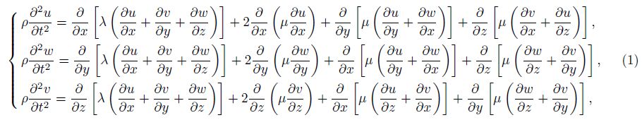
Only considering elastic waves in two dimensions,Eq.(1) can be rewritten as
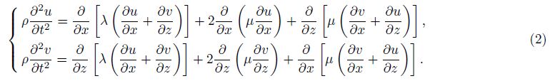
Eq.(2) can be written in the following simple form:
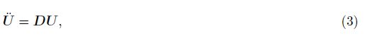
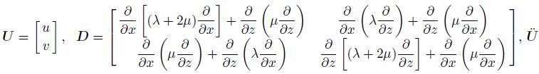 is the second order derivative of displacement vector with respect to time.
Introducing generalized momentum p = $\dot U$ and generalized coordinate q = U,the 2n-dimensional phase space Z = (p,q) in terms of generalized momentum and coordinate advances in time domain can be expressed in the following Hamilton canonical equation:
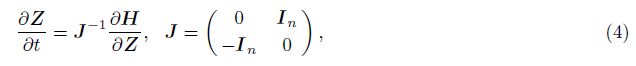

H represents the total energy of the dynamic system. If H is not related to time,system energy is conservative. Under the symplectic transform,the canonical form of Eq.(4) preserves. The basic theorem of Hamilton dynamics is that the phase at time t can be obtained by canonical transform in terms of H and phase at original time,which can be written as

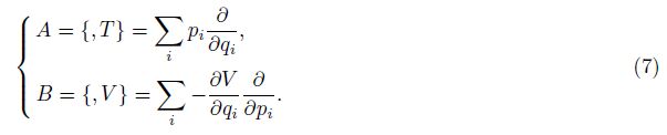
Canonical transform Eq.(6) can preserves symplectic structure of the Hamilton system,that is to say,the 2-differential form does not change at each time step. From Eq.(5),we find that seismic wave equation is a separable Hamilton system. For a separable Hamilton system,it is easy to construct symplectic schemes with accuracy of any order[38]. To construct symplectic schemes simply,we define Lie operators[24, 25] A and B in terms of T(p) and V (q),respectively,which can be written as
Third or higher order schemes can improve accuracy,but huge computational cost hiders the implementation of high-order schemes in seismic simulations. In order to meet the need of practical applications,we design a second-order symplectic scheme as follows:
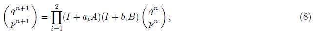
In Eq.(8) four coefficients need to satisfy three equations,thus Eq.(8) has one degree of freedom. Using BCH formula[24, 25, 26] for exponential operator expansion,we obtain optimal coefficients based on minimum error truncation; the process is discussed in the appendix A. The optimal coefficients are

The traditional FDM has a high efficiency in seismic wave simulations,but suffers from numerical dispersion when spatial increment is large[39, 40]. Preserving the advantages of the FDM and suppressing its drawbacks is a focus of this paper. We introduce the generalized Shannon convolutional differential operator (GCD) to calculate spatial derivatives.
The generalized Shannon singular function can be defined as[22]
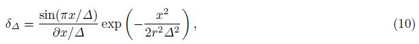
When △ → 0,Eq.(10) is a good candidate of Delta function. The generalized Shannon interpolation function can be written as

For an arbitrary discrete sequence {u(xi)},the spatial derivate of u(x) can be written as
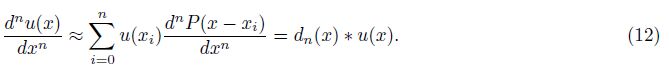
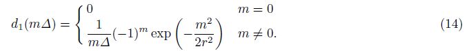
Solving Eq.(11) numerically involves calculation of the first-order,second-order and mixed spatial derivatives. The first-order operator is
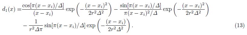
If the spatial increment is x = m△,Eq.(13) can be expressed as
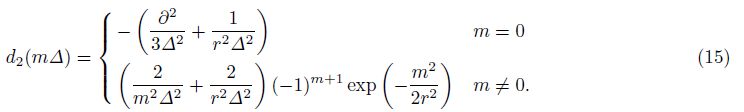
We can obtain the second-order operator in a similar way,which is
Eqs.(14) and (15) are long operators,which involve the values at all spatial nodes. In practical calculation, we need to truncate long operators into short operators. To avoid the Gibbs phenomenon,we choose the Hanning window to truncate the operators,and the window function can be written as
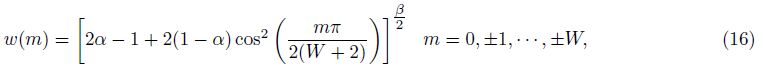
The truncated operator is
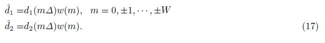
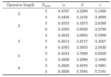
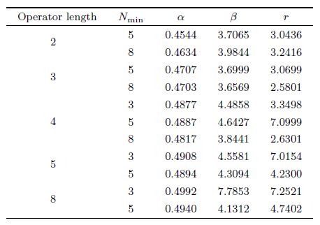
From Eq.(17),we can find that the first-order operator is symmetric,while the second-order operator is of anti-symmetry. To ensure the minimum error of group velocity and energy conservation,the first-order operator needs no change,while we must revise the value of the middle node of the second-order operator to be equal to the opposite value of the sum of the value of the other nodes[20]. Three coefficients α,β,r need to be determined in Eq.(17). Upon the derivative approximating principle,we obtain optimal coefficients for Eq.(17),which are presented in Table1 and 2. The process of derivation can be found in Appendix B. Table1 and 2 show that the optimal coefficients are determined by the minimal sample rate and the operator length. In practical seismic simulations,we can choose different coefficients under specific situations to obtain high accuracy. In practical application,the coefficients of Nmin = 5 can satisfy most cases. Pursuing the high accuracy in the high wave number domain and choosing smaller Nmin will lead to larger errors in the low wave number domain. To balance the efficiency and accuracy,we choose the operator with W = 4,Nmin = 5 in seismic wave simulations.
| Table 1 Optimal coefficients of window function for first-order GCD |
| Table 2 Optimal coefficients of window function for second-order GCD |
We use the first-order derivative of f(x) to analyze the accuracy of GCD in calculating spatial derivatives. f'(x) can be transformed into ikxF(kx) by Fourier transform. F(kx) is phase of f(x) under Fourier transform,and the filter response of the spatial derivative under Fourier transform is ikx. The filter response of GCD is
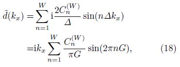
The filter response rate of GCD is Rk =$\sum\limits_{n = 1}^W {\frac{{C_n^{(W)}}}{{\pi G}}} \sin (2\pi nG)$.Fig.1 shows the filter response rates of FDM and GCD,which indicates that GCD with radius equal to 4 (GCD4) is more accurate than FDM with radius equal to 5 (FDM5).

|
Fig.1 Comparison of filter response ratios of GCD and FDM operators |
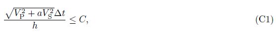
Using OSGCD for seismic simulations,the time interval and spatial increment should satisfy some proportional relation to keep the algorithm stable. Following literature [30],we define the stability condition as
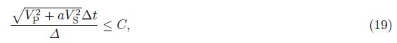
In Appendix C,derivation process is present in a 2D case,and the result is a = 0.6986,C = 0.8138.
3 NUMERICAL EXPERIMENTS 3.1 2D Infinite Homogeneous ModelWe design a 2000 m×2000 m homogeneous model (Fig.2) to test the efficiency and accuracy of OSGCD in practical seismic wave simulations. Four methods are employed to compare with our method,which are (1) PRK Lobatto III A-III B[32, 33, 34, 35] in combination with GCD (PRK-GCD),(2) Iwatsu three-stage and third-order symplectic scheme[15, 28, 29, 30, 36] in combination with GCD (TO-GCD),(3) optimal two stage and second order symplectic scheme in combination with SCD[15, 28, 29, 41] (OS-SCD) and (4) optimal second-degree and secondorder symplectic scheme in combination with FDM (OS-FEM). In this numerical experiment,we choose VP=2000 m/s,VS=1250 m/s and ρ=2000 kg/m3. A vertical point-focus source is used,which is Ricker wavelet with a peak amplitude spectrum at 30 Hz,and located at the center of the model. One receiver R1 is located at (1200 m,1200 m). The spatial increment is 5 m,and the time increment is 0.5 ms. The numerical tests are implemented on the same computer with Intel (R) Core (TM) i5-2320 CPU and 16 GB RAM. The results are shown in Fig.3,Fig.4,and Table3, respectively.

|
Fig.2 2-D half infinite space for elastic wave propagation |

|
Fig.3 (A) Comparison of waveforms generated by OSGCD, PRK-GCD and TO-GCD; (B) Comparison of absolute errors generated by three different time discretization methods |

|
Fig.4 (A) Comparison of waveforms generated by OSGCD, OS-SCD and OS-FDM; (B) Comparison of absolute errors generated by three different spatial derivative methods |
| Table 3 Comparison of computational efficiency of five methods |
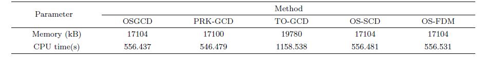
From Fig.3a,one can find that the waveforms generated by OSGCD,PRK-GCD,and TO-GCD are very close to the analytical waveform,which means that numerical solutions modeled by these three methods can obtain credible results,while from Fig.3b,it is clear that the absolute errors of both OSGCD and TO-GCD are extremely close to each other,and very smaller than PRK-GCD; Table3 shows that TO-GCD consumes largest memory and CPU time to achieve high accuracy,which means that TO-GCD is less efficient than OSGCD in seismic simulations. We also compare the waveforms calculated by OSGCD,OS-SCD,and OS-FDM as shown in Fig.4. Fig.4a shows that three derivative methods are valid,but from absolute errors,as shown in Fig.4b, OSGCD is more accurate than the other two methods,while the computation costs are almost the same among these three methods. The comparisons demonstrate that OSGCD has great advantages over the other four methods in computational costs and numerical accuracy.
3.2 Long-Time SimulationsTo investigate the ability of OSGCD in long-time simulations,a 2D 6000 m×6000 m homogeneous model with rigid boundaries is constructed. We use OSGCD and the popular Runge-Kutta FDM (RK-FDM) to simulate SH wave propagation. A shear source,which is a Ricker wavelet with a peak spectrum at 20 Hz,is located at the center of the model. The velocity of P-wave is 3000 m/s; the velocity of S-wave is 2000 m/s; the mass density is 2000 kg/m3. The spatial increment is 10 m and the time increment is 1 ms.
Figure5 displays the snapshots of the wavefield simulated by these two methods at different time instants. From Fig.5(a,b),it can be found that in short-time simulations these two methods result are in the largely same snapshots. But as the time increases,the wavefront in Fig.5c is blurred severely,while the wavefronts in Fig.5d are still quite clear,which means that OSGCD is quite suitable for long-time seismic simulations.

|
Fig.5 Snapshots of wavefields generated by RK-FDM(a)(c) and OSGCD(b)(d); (a) and (b) time step=1500; (c) and (d) time step=25000 |
The media of the real earth are strongly heterogeneous. It is necessary to investigate the ability of our methods for simulating seismic wave in strongly heterogeneous media. We choose the 3840 m×1210 m Marmousi model,which contains continuous and discontinuous elastic parameter changes,and the velocity profile of Pwave is shown in Fig.6. The velocity ranges from 1500 m/s to 5500 m/s; the S-wave velocity is VS = VP/$\sqrt 3 $ the mass density is obtained by Gardner formula ρ = 310 × VP0.25 [43]. A point-explosive source is located at centre of the model,which is a Ricker wavelet with an amplitude spectrum peak at 30 Hz. A receiver is located at (192,91) node point. The spatial interval is 10 m and the temporal interval is 1.0 ms. The PML boundary condition[44] is adopted to avoid boundary reflection. We compare OSGCD with PSM in this experiment.

|
Fig.6 Marmousi velocity model |
The snapshots of wave field at t=0.25 s in terms of the vertical displacement component are shown in Fig.7,and seismic records are presented in Fig.8. It can be found that there is no obvious difference between OSGCD and PSM in seismic wave simulation in the heterogeneous media. Because of the dramatic disturbance of elastic parameters of the model in Fig.6,we can see clearly the diffraction waves and scattered waves in Fig.7. This experiment indicates that OSGCD can generate creditable results when simulating seismic waves in strongly heterogeneous media.

|
Fig.7 Snapshots of wave field at 0.25s in Marmousi model (a) is generated by PSM; (b) is generated by OSGCD. |
Transforming the seismic wave equation in terms of displacement into the Hamiltonian system,we design a new symplectic scheme by means of Lie operators. The optimal coefficients are obtained based on minimum error truncation. We develop an optimal convolutional differential operator to calculate spatial derivatives. The stability conditions of OSGCD are presented. In numerical experiments,we compare our methods with traditional methods in various aspects. The results demonstrate that the performance of OSGCD is more efficient and can reduce computing costs dramatically. Our method is very suitable for long-time computation for its structure preserving properties. In simulating seismic waves in heterogeneous media,the results obtained by the new method are nearly the same as the PSM; the seismograms contain lots of information which is especially useful for determining geological structure.
5 Appendix ADefining reciprocal relations[45] [A,B] = AB - BA and [A,B,A] = [A,[B,A]],we have

By Baker-Campell-Hausdroff (BCH) formula, we obtain the expansion of W in the following form:
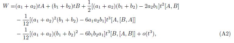
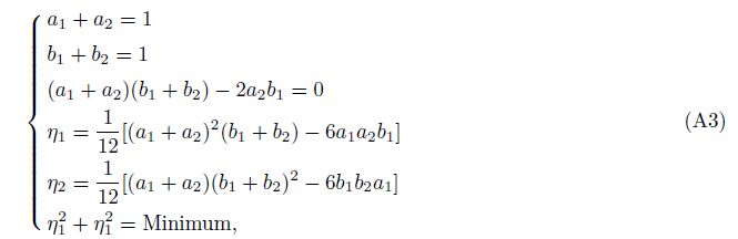
From (A3),we obtain ${a_1} = 1 - \frac{1}{{\sqrt 2 }},{a_2} = \frac{1}{{\sqrt 2 }},{b_1} = 1 - \frac{1}{{\sqrt 2 }},{b_2} = \frac{1}{{\sqrt 2 }}$.
6 Appendix BConsidering the following 2D harmonic plane wave:


|
Fig.8 Seismograms in Marmousi model (a) is generated by PSM; (b) is generated by OSGCD. |
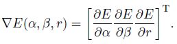
The numerical derivative of (B1) calculated by GCD is ${\hat d_1}$ * P(x,z,w),and the analytic derivative of (B1) is P'(x,z,w). The numerical derivative should approach as close as possible to the analytic derivative,and we have the following object function:

Eq.(B2) is nolinear optimization problem,and we construct the following iteration based on the steepest descent method:

 7 Appendix C
We set the stability conditions of M1,M2,and M3 to be


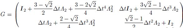 ; I2 is two level identity matrix,Λ2 is two level matrix and can be expressed as Λ2 = (aij)2×2,a11 = VP2 kx2 + VS 2 kz2 ,a12 = (VP2 - VS 2 )kxkz,a21 = a12,a22 = VS 2 kx2 + VP2kz2 ,kx = k sin θ,kz = k cos θ,k = $\frac{\pi }{\Delta }$ and 0 ≤ θ ≤ 2π. We define r =$\frac{{{V_P}}}{{{V_S}}}$,α = $\frac{{{V_P}\Delta t}}{h}$and G
is a function of the variables r,α. If and only if the spectral radius of matrix G is less than or equal to 1,(C3) converges; so G must satisfy the following equation:
; I2 is two level identity matrix,Λ2 is two level matrix and can be expressed as Λ2 = (aij)2×2,a11 = VP2 kx2 + VS 2 kz2 ,a12 = (VP2 - VS 2 )kxkz,a21 = a12,a22 = VS 2 kx2 + VP2kz2 ,kx = k sin θ,kz = k cos θ,k = $\frac{\pi }{\Delta }$ and 0 ≤ θ ≤ 2π. We define r =$\frac{{{V_P}}}{{{V_S}}}$,α = $\frac{{{V_P}\Delta t}}{h}$and G
is a function of the variables r,α. If and only if the spectral radius of matrix G is less than or equal to 1,(C3) converges; so G must satisfy the following equation:


We would like to thank the two anonymous reviewers for their careful reading and valuable comments on the manuscript. This work was supported by the National Natural Science Foundation of China (41174047, 40874024 and 41204041).
| [1] Chen J B, Qin M Z. Ray tracing by symplectic algorithm. Journal of Numerical Methods and Computer Applications (in Chinese), 2000, 21(4): 255-265. |
| [2] Červeny V. Seismic Ray Theory. Cambridge: Cambridge University Press, 2001. |
| [3] Pao Y H, Varatharajulu V. Huygen's principle, radiation conditions, and integral formulas for the scattering of elastic wave. J. Acoust. Soc. Am., 1976, 59(6): 1361-1371. |
| [4] Ursin B. Review of elastic and electromagnetic wave propagation in horizontally layered media. Geophysics, 1983, 44(8): 1063-1081. |
| [5] Mou Y G, Pei Z L. Seismic Numerical Modeling for 3-D Complex Media (in Chinese). Beijing: Petroleum Industry Press, 2005. |
| [6] Dong L G, Ma Z T, Cao J Z. A study on stability of the staggered-grid high-order difference method of first-order elastic wave equation. Chinese J. Geophys. (in Chinese), 2000, 43(6): 856-864. |
| [7] Zhang M G, Wang M Y, Li X F, et al. Finite element forward modeling of anisotropic elastic waves. Progress in Geophysics (in Chinese), 2002, 17(3): 384-389. |
| [8] Gazdag J. Modeling of the acoustic wave equation with transform methods. Geophysics, 1981, 46(6): 854-859. |
| [9] Komatitsch D. Spectral and spectral-element methods for the 2D and 3D elastodynamics equations in heterogeneous media. Paris, France: Institut de Physique du Globe, 1997. |
| [10] Carcione J M, Herman G C, ten Kroode A P E. Seismic modeling. Geophysics, 2002, 67(4): 1304-1325. |
| [11] Yang D H, Song G J, Lu M. Optimally accurate nearly analytic discrete scheme for wave-field simulation in 3D anisotropic media. Bull. Seism. Soc. Am., 2007, 97(5): 1557-1569. |
| [12] Bayliss A, Jordan K E, Lemesurier B J, et al. A fourth-order accurate finite-difference scheme for the computation of elastic wave. Bull. Seism. Soc. Am., 1986, 76(4): 1115-1132. |
| [13] Fornberg B. The Pseudospectral method: Comparisons with finite differences for the elastic wave equation. Geophysics, 1987, 52(4): 483-501. |
| [14] Fornberg B. The Pseudospectral method: Accurate representation of interfaces in elastic wave calculations. Geophysics, 1988, 53(5): 625-637. |
| [15] Li X F, Wang W S, Lu M W, et al. Structure-preserving modelling of elastic waves: a symplectic discrete singular convolution differentiator method. Geophys. J. Int., 2012, 188(3): 1382-1392. |
| [16] Mora P. Elastic Finite Differences with Convolutional Operators. California: Stanford Exploration Project Report, 1986: 277-290. |
| [17] Holberg O. Computational aspects of the choice of operator and sampling interval for numerical differentiation in large-scale simulation of wave phenomena. Geophysical Prospecting, 1987, 35(6): 629-655. |
| [18] Zhou B, Greenhalgh S. Seismic scalar wave equation modeling by a convolutional differentiator. Bull. Seism. Soc. Amer., 1992, 82(1): 289-303. |
| [19] Zhang Z J. Teng J W. Yang D H. The convolutional differentiator method for numerical modeling of acoustic and elastic wave-field. Acta Seismologica Sinica (in Chinese), 1996, 18(1): 63-69. |
| [20] Dai Z Y, Sun J G, Cha X J. Seismic wave field modeling with convolutional differentiator algorithm. Journal of Jilin University (Earth Science Edition) (in Chinese), 2005, 35(4): 520-524. |
| [21] Long G H, Zhao Y B, Zhao J F. Optimal Shannon singular kernel convolutional differentiator in seismic wave modeling. Acta Seismologica Sinica (in Chinese), 2011, 33(5): 650-662. |
| [22] Wei G W. Quasi wavelets and quasi interpolating wavelets. Chemical Physics Letters, 1998, 296(3-4): 215-220. |
| [23] Qian L W. On the regularized Whittaker-kotel'nikov-Shannon sampling formula. American Mathematical Society, 2002, 131(4): 1169-1176. |
| [24] Li R, Wu X. Two new Fourth-order Three-stage symplectic integrators. Chin. Phys. Lett., 2011, 28(7): 070201, doi: 10.1088/0256-307X/28/7/070201. |
| [25] Li R, Wu X. Application of the fourth-order three-stage symplectic integrators in chaos determination. Eur. Phys. J. Plus, 2011, 126(8): 73-80. |
| [26] Casas F, Murua A. An efficient algorithm for computing the Baker-Campbell-Hausdorff series and some of its applications. Technical report, Universitat Jaume I, 2008. |
| [27] Ruth R D. A canonical integration technique. IEEE Transactions on Nuclear Science, 1983, 30(4): 2669-2671. |
| [28] Iwatsu R. Two new solutions to the third-order symplectic integration method. Physics Letter A, 2009, 373(34): 3056-3060. |
| [29] Li Y Q, Li X F, Zhu T. The seismic scalar wave field modeling by symplectic scheme and singular kernel convolutional differentiator. Chinese J. Geophys. (in Chinese), 2011, 54(7): 1827-1834. |
| [30] Li Y Q, Li X F, Zhang M G. The elastic wave fields modeling by symplectic discrete singular convolution differentiator method. Chinese J. Geophys. (in Chinese), 2012, 55(5): 1725-1731. |
| [31] Wang W S, Li X F. A new solution to the third-order non-gradient symplectic integration algorithm. J. Wuhan Univ. (Nat. Sci. Ed.) (in Chinese), 2012, 58(3): 221-228. |
| [32] Luo M Q, Liu H, Li Y M. Hamiltonian description and symplectic method of seismic wave propagation. Chinese J. Geophys. (in Chinese), 2001, 44(1): 120-128. |
| [33] Sun G. A class of explicitly symplectic schemes for wave equations. Mathematica Numerica Sinica (in Chinese), 1997, (1): 1-10. |
| [34] Ma X, Yang D H, Zhang J H. Symplectic partitioned Runge-Kutta method for solving the acoustic wave equation. Chinese J. Geophys. (in Chinese), 2010, 53(8): 1993-2003. |
| [35] Ma X, Yang D H, Liu F Q. A nearly analytic symplectically partitioned Runge-Kutta method for 2-D seismic wave equations. Geophys. J. Int., 2011, 187(1): 480-496. |
| [36] Li X F, Li Y Q, Zhang M G, et al. Scalar seismic-wave equation modeling by a multisymplectic discrete singular convolution differentiator method. Bull. Seism. Soc. Am., 2011, 101(4): 1710-1718. |
| [37] Feng K, Qin M Z. Symplectic Geometric Algorithm for Hamiltonian Systems (in Chinese). Hangzhou: Zhejiang Science & Technology Press, 2003. |
| [38] Suzuki M. General theory of higher-order decomposition of exponential operators and symplectic integrators. Phys. Lett. A, 1992, 165(5-6): 387-395. |
| [39] Dablain M A. The application of high-order differencing to the scalar wave equation. Geophysics, 1986, 51(1): 54-56. |
| [40] Fei T, Larner K. Elimination of numerical dispersion in finite-difference modeling and migration by flux-corrected transport. Geophysics, 1995, 60(6): 1380-1842. |
| [41] Long G H, Li X F, Zhang M G. The application of convolutional differentiator in seismic modeling based on Shannon singular kernel theory. Chinese J. Geophys. (in Chinese), 2009, 52(4): 1014-1024. |
| [42] Smith G D. Numerical Solution of Partial Differential Equations: Finite Difference Methods. Oxford: Glarendon Press, 1978. |
| [43] Li X F, Li X F. Numerical simulation of seismic wave propagation using convolutional differentiator. Earth Science-Journal of China University of Geosciences (in Chinese), 2008, 33(6): 861-866. |
| [44] Berenger J. A perfectly matched layer for the absorption of electromagnetic waves. J. Comput. Phys., 1994, 114(2): 185-220. |
| [45] Xu J, Wu X. Several fourth-order force gradient symplectic algorithms. Research in Astronomy and Astrophysics, 2010, 10(2): 173-188. |
| [46] Jo C H, Shin C, Suh J H. An optimal 9-point, finite-difference, frequency-space, 2-D Scalar wave extrapolator. Geophysics, 1996, 61(2): 529-537. |