1 INTRODUCTION

Magnetic anomalies can provide information on structure of crust both exposed on the ground surface or buried below. Magnetic anomaly maps illuminate tectonics and contain evidence for geothermal evolution. Compared to gravity anomalies,in which the density of the source body is a scalar quantity,a magnetic anomaly has more complexity. It depends on the characteristics of the magnetic source itself,as well as on the direction of magnetization and on the direction in which the field is measured. If ignoring the influence of remnant magnetization,magnetic anomalies located anywhere other than at the magnetic poles are asymmetric even when the magnetic source distribution is symmetrical,completely different from gravity anomalies. To make comprehension of magnetic maps easy,Baranov^{[1, 2]} first introduced the operator of reduction to the pole (RTP) in 1957. This method transforms the observed magnetic anomaly into the anomaly that is measured in the case the magnetization and ambient fields are both vertical. Bhattacharyya^[3] made it clear that RTP can be accomplished more expediently by harmonic analysis. Kanasewich and Agarwal^[4] modified the Bhattacharyya’s method to take advantage of the fast Fourier transform (FFT) algorithm. Gunn^[5] showed that RTP is linear transformations of magnetic fields by multiplying the Fourier transform of the anomaly by the frequency response of a filter with a closed form formula. RTP has become a standard part of data processing as a simple filtering operation performed in the wave number domain by multiplying the Fourier transform of the observed magnetic field with the RTP operator in the wave number domain.

However,the RTP operator has several well-known problems. The operator becomes unstable at lower magnetic latitudes,in addition to the problem of unknown remnant magnetization. As the magnetic latitude approaches the equator,the RTP filtering operation becomes unbounded because of a singularity that appears when the azimuth of the body and the magnetic inclination both approach zero. Baranov^[1] suggested that the magnetic dip for RTP should be more than 30 degrees. Later Baranov and Naudy^[2] proposed the smallest inclination is 16.5 degrees in their algorithm. Silva^[6] pointed out that the FFT technique for RTP has a poor performance at low magnetic latitudes less than 15 degrees,which is of no practical use due to a sharply increasing instability toward the magnetic equator. The direct method to overcome this problem is reducing anomalies measured at low magnetic latitudes to the equator rather than the pole^[7]. This approach overcomes the instability,but anomaly shapes are difficult to interpret. Silva^[6] used an equivalent source technique for reducing magnetic anomalies to the pole at any latitudes. Hansen and Pawlowski^[8] designed an approximately regulated filter usingWiener techniques for reduction to the pole at low magnetic latitudes. Keating and Zerbo^[9] modified the Wiener filtering technique for reduction to the pole at low magnetic latitudes by introducing a simple noise model. Li and Oldenburg[10^-11] proposed a technique that attempts to find the RTP field under the general framework of an inverse formulation both in the space domain and wave number domain. In China,Zhang^[12] designed several stable filters for formulating stable approximations of the RTP operator. Yao^{[13, 14]} also designed a suppression filter and damper filter for reduction to the pole at low magnetic latitudes to suppress specific frequencies in the wave number domain. Luo^[15] proposed a novel inversion method by probability tomography and realized RTP operator at low magnetic latitudes. Luo^[16] also proposed an iterative formula for RTP at the magnetic equator. Analytic signal theory is another method for interpretation of total magnetic field data at low magnetic latitudes. MacLeod^[17] has discussed the method. But unlike the 2-D analytic signal,the analytic signal in 3-D is not independent of direction of magnetization,nor does it represent the envelope of both the vertical and horizontal derivatives in all possible directions of the normal magnetic field and source magnetization.

The standard RTP operator assumes that the directions of the normal magnetic field and the magnetization are constant over the entire region,but it is certainly not valid for large-scale regional magnetic anomalies. The standard RTP processing may distort the magnetic anomalies over the entire area for large-scale surveys. Arkani-Hamed^[18] presented an equivalent-layer scheme for reducing a grid of total field magnetic data to the pole,in which the field and magnetization directions vary. The method presented by Arkani-Hamed was named differential reduction to the pole (DRTP). Swain^[19] modified the DRTP algorithm to improve the stabilization at low magnetic latitudes. Then Arkani-Hamed^[20] proposed a new modification to the DRTP,which preserves the correct RTP anomalies over almost the entire area except for very low latitudes. Cooper and Cowan^[21] suggested a simple algorithm for DRTP which employs a Taylor series expansion in the space domain,but this algorithm has singularity at the geomagnetic equator. In China,the common approach is to divide the area into many small subareas,which allows the standard RTP processing to be applied to each subarea and the resulting RTP maps compiled into a large-scale DRTP map. But this approach introduces errors into the final composite map and the signatures specified by wavelengths longer than the dimension of individual subareas will be lost in the processing.

Though many geophysicists have modified the RTP operator and presented perfect results for practice data processing,the RTP and DRTP operators in the wave number domain still face difficulties in theory. The difficulties may be caused by Fourier transform,for example the RTP filter is a phase transformation that is more complex than the downward continuation filter. Chai^{[23, 24]} suggested a shift sampling method for Fourier transform computation and applied it to RTP at low magnetic latitudes. This work proposes a new scheme for RTP by using Hartley transform. This method also encounters problems at the low magnetic latitudes. This paper addresses these difficulties and suggests to slightly increase the inclination of the normal magnetic field at low latitudes to suppress the north-south trending features. Calculations on theoretical models and real data demonstrate the RTP operator in the Hartley domain is an effective algorithm.

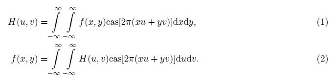
2 METHODOLOGY 2.1 Hartley Transform and Its Property

An integral transform similar to the Fourier transform was presented by Hartley^[25] in 1942. Bracewell^[26] called the integral transform Hartley transform and introduced the formula for discrete Hartley transform (DHT). Further,Bracewell suggested that the Hartley transform is as fast as or faster than the fast Fourier transform (FFT) and can be used anywhere the Fourier transform is applied. Scholars have proposed fast Hartley transform (FHT) algorithm^{[27, 28]}. The fast Hartley transform minimizes the CPU time and occupies less memory compared to the fast Fourier transform,and extensive results of research and application on Hartley transform published by Institute of Electrical and Electronics Engineers (IEEE). There are two different versions of kernels associated with the 2-D Hartley transform,and Sundararajan^[29] investigated their relation. According to the Brancewell’s^[30],this work adopts a standard form of the two-dimensional Hartley transform which is expressed as^[31]

Their discrete forms are where cas(θ) = cos θ + sin θ. The DHT could be made strictly symmetrical by changing the factor M-1N-1 in the definition of the DHT into M^-1/2N^-1/2. Then changing the definition of the inverse DHT to include the same factor,we would have a strictly symmetrical transformation. Hartley ensured the symmetry of his original relations by such means^[30]. A convenience of the 2-D Hartley transform is that it may be presented as a single diagram representing the full spectral of analysis for an image. Whereas the Fourier transform of an image,which hardly ever published,requires two diagrams,either for the real and imaginary parts,or for the amplitude and phase. The phase spectra have almost never been used in potential field data processing,in most cases only using the amplitude spectra. The convenience of the 2-D Hartley transform spectra may provide an effective tool for the spectral analysis.

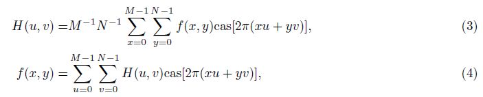
To derive the formula for reduction to the pole in the Hartley domain,we first give some properties without proof as follows.

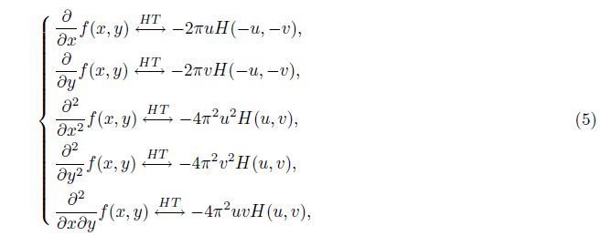
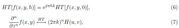
where HT means Hartley transform and H(u,v) = HT[f(x,y)]. In addition,the expressions for potential field data upward continuation and vertical derivative calculating are where h ＜ 0 and is the wave number. The proving for Eq.(6) can refer to formula for upward continuation of profile potential field data by Hartley transform^[32],and the appendix shows the proof of it.

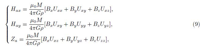
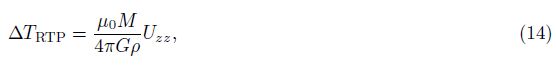
2.2 Hartley Transform for RTP

If the anomalous field is small compared to the ambient field,then the total field anomaly is projection of anomalous field onto the normal magnetic field. The total field anomaly is given by

According to the Poisson’s relation the total field anomaly can be expressed as where H_ax,H_ay and Z_a are the x,y,and z components of the anomalous field,respectively,B₀ = {B_x,B_y,B_z} is the geomagnetic field unit vector,μ₀ is the vacuum permeability,M is the magnetization intensity,U is the gravitational potential. G is the gravitational constant,and ρ is the density.

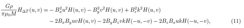
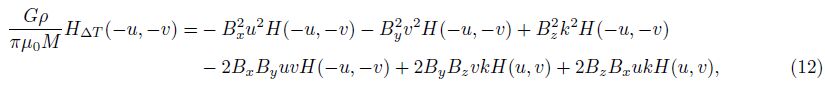
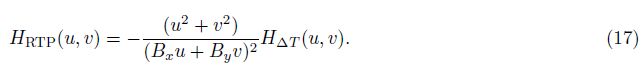
Using Eq.(5) to (7) and taking the Hartley transform of the resulting Eq.(10) yield

and if let u = -u,and v = -v,then there is where H△T (u,v) is the Hartley transform of △T(x,y),H(u,v) is the Hartley transform of U,u and v are wave numbers,and .

According to Eqs.(11) and (12),it is easy to obtain

At the north geomagnetic pole,where B₀ = {0,0,1},Eqs.(9) and (10) reduce to whose Hartley transform is The RTP result is calculated as where R = B_z² k² - (B_xu + B_yv)²,P = 2B_zk(B_xu + B_yv) and T = B_z²k² + (B_xu + B_yv)2. Finally,making the Hartley transform of resulting Eq.(16),we obtain the RTP field. Eq.(16) contains two parts. Two filters are applied to the spectra of magnetic anomalies and the phase filtering is similar to the Fourier transform.

2.3 Discussion for Low Latitudes

If the magnetization and ambient field are both horizontal,i.e. B_z = 0,then

The RTP filter including no imaginary part is equivalent to the filter in the Fourier domain. The RTP method by Hartley transform is also unstable. To better understand the difficult at low latitudes,we convert Eq.(16) into polar coordinates: where and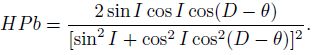

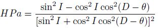
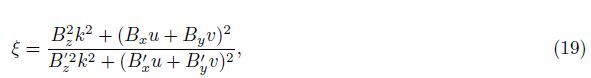
Eq.(18) identifies the behavior of filter as a function of spectral azimuth. Fig.1 shows the behavior of HPa filter and HPb filter between zero and 360 degrees for a magnetization azimuth of zero degree and magnetization inclinations between 5 and 15 degrees. We observe the rapid increase of HPa and HPb at or near azimuths 90 and 270 degrees as the inclination approaches zero degrees. The large values of HPa occur only around the spectral azimuth given by θ = D ± 90 degrees and for inclinations close to zero degree. The curves of HPa are similar to Fig.1 given by Mendonca and Silva^[33]. But the curves of HPb in Fig.1 show its phase is completely different from the HPa filter. As two kinds of amplitude filters,HPa and HPb work together to achieve a similar phase filtering in the Fourier domain. The filters of HPa and HPb in the wave number domain at low latitudes become unstable in a wedge-shaped segment. Yao^{[13, 14]} suggested a damping filter in a wedge-shaped segment within 12 degrees as a compromise operator considering the instability filters of HPa and HPb. The simplest effective solution to this problem is to modify the filters of HPa and HPb so as to limit the amount of north-south amplification. This modification needs to consider three aspects. Firstly,the modification should be slight,otherwise the spectra will lose the characteristics of transformation. Secondly,the modification should be smooth and the filter smoothly tapers the RTP operator. Thirdly,the modification for two amplitude filters in Eq.(16) or (18) should be the same. Peng^[34] modified the imaginary part of the damping filter given by Yao^[14] which actually considers the third aspect. Attempts were made by MacLeod^[17],Swain^[19],and Arkani-Hamed^[20] to suppress the singularity by using the procedure in Geosoft’s MAGMAP software,which reduces the amplitude of the RTP operator. The filter used is

where B'₀= {B' _x ,B'_y ,B'_z } is the pseudo-inclination unit vector. This simplest effective solution is actually assuming a new direction of magnetization different from the normal magnetic field,while at low latitudes introducing a relatively large angle of magnetization. After the modification,the RTP filters in the Hartley domain are MHPa = HPaζ and MHPb = HPbζ. Fig.2 shows the behavior of MHPa filter and MHPb filter between zero and 360 degrees for a magnetization azimuth of zero degree and magnetization inclinations between 0 and 2.5 degrees. The pseudo-inclination is 10 degrees in Fig.2. It clearly shows that the pseudo-inclination can make the filter curves stable. However,although the Eq.(19) certainly stabilizes the RTP,and it does in fact alter the phase. Take the Fourier transform of the curves in Fig.1 and Fig.2,we find the phase of the filter curves has been slightly changed. This phase change is very small,which is why we select Eq.(19) to overcome singularity and instability at low latitudes.

3 THEORETICAL EXAMPLES

To test the proposed method,this work reduces the total field anomalies simulated at different latitudes using a simple synthetic model that was designed by Hansen and Pawlowski^[8]. This model is a rectangular body with 20 m in both x- and y-directions,a thickness of 2 m,and top at 1 m below the ground surface. The magnetization is induced only,having an intensity of 0.35 A/m. All the total field anomalies are calculated using a 64×64 mesh with interval 1 m in each direction. Fig.3a shows the horizontal slice of the model,and Fig.3b shows its true RTP field produced by this model. Fig.4 shows two RTP examples by Hartley transform. The inclinations are 60 degrees and 15 degrees,respectively,which are typical mid- high latitudes and low latitudes. It is clear that the RTP results (Fig.4b or Fig.4d) are consistent with the theoretical field (Fig.3b). It should be noted that the buried model is very shallow and the actual error for transformation is large. In the processing above,no any other methods are used to improve the RTP results,including data expanding or filtering.

As a low-latitude example,this work reduces the total field anomalies simulated at the equator (Fig.5a) using the model in Fig.3a. Figure5b shows the RTP result by Hartley transform,where the pseudo-inclination is 20 degrees. Compared with the prevous work^[34],this result is acceptable. The pseudo-inclination method is the simplest effective solution,though the reduction effect is not as perfect as the algorithm of reduction to the pole at the geomagnetic equator proposed by Luo^[16]. To illustrate the impact of the pseudo-inclination at low latitudes,these anomalies (Fig.5a) at different pseudo-inclination conditions are reduced. Fig.6a shows the RTP result with pseudo-inclination 3 degrees. It clearly shows the central high above the causative body and four negative side lobes. There is,however,visible elongation in the north-south direction. The larger degree of pseudo-inclination,the RTP field is more stable. The RTP field exhibits the similar characteristics of the total field anomalies in large pseudo-inclination degree conditions. Fig.6b shows the RTP result for pseudo-inclination 60 degrees. Fig.6b and Fig.5a are similar in intensity but opposite in signs. They are approximately phase reversal 180 degrees. The phase reversal method has been applied to magnetic interpretation at low attitudes. Guo^[35] adopted the ‘reverse tangent’ technique of △T profile negative magnetic anomalies for calculating buried depths of magnetic plates at low magnetic latitudes. Thus,the coefficient tables at high latitudes can be used to calculate the buried depth of the magnetic plate which usually produces △T profile negative magnetic anomalies at low latitudes directly. In addition,Fang^[36] analyzed the relations between Z_a,Ha and △T under different magnetized conditions and suggested a phase reversal 180 degree method for interpreting magnetic anomalies in the South China Sea. Fig.6b shows that the phase reversal method is an approximate RTP processing at low latitudes. It illustrates that Luo^[16] adopted the phase reversal 180 degree as mapping function in reduction to the pole at the geomagnetic equator is reasonable.

4 REAL DATA EXAMPLE

Theoretical model calculations have shown that the effect of reduction of magnetic data to the pole by Hartley transform. Here an example of real data at low latitudes is presented,i.e. the South China Sea at low latitudes with the dip nearly zero. As both the area and span of this place is not large,and the direction of the core field does not vary. The RTP method proposed in this paper,Eq.(19),can be used directly to calculate it. The pseudo-inclination is 20 degrees. Fig.7a and Fig.7b show the total field anomalies and the RTP field,respectively. Comparison indicates that the magnetic fields before and after RTP processing change greatly both in shape and intensity. The RTP field remains stable and has no distortion. The data shown in Fig.7a has been processed with a series of methods,although previous processing for RTP is focused on inverting the original magnetic anomalies. Fig.7b is consistent with previous RTP results. The real data processing shows that it can directly implement RTP operator by Hartley transform at low latitudes with the pseudo-inclination method.

5 CONCLUSIONS

This paper presents a new algorithm of reduction to the pole by Hartley transform. The method combined with the pseudo-inclination is convenient for routinely computation at low latitudes. Being a real valued function and fully equivalent to the Fourier transform,the Hartley transform is more efficient and economical than its progenitor. Thus,the RTP processing by Hartley transform will be also more efficient and economical,which may allow each grid node to implement the RTP operator with different inclinations and declinations. The method would play an active role in interpretation of magnetic anomalies.

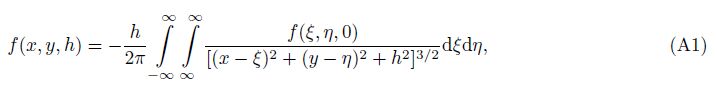
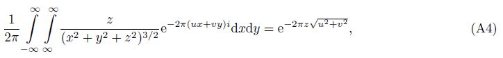
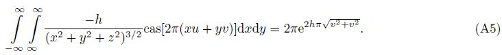
6 Appendix

Potential data at two observation heights are related by the upward continuation operation:

where f(x,y,h) and f(x,y,0) are the potential data at two different heights (h ＜ 0). Eq. (A1) can be written as a convolution form: As the function -h/(x²+y²+h²)3/2 is an even function,its Hartley transform satisfies the convolution theorem similar to Fourier transform. Thus,the Hartley transform of Eq.(A2) is where HT denotes the Hartley transform. With a basic integral formula we can get the Hartley transform of -h/(x² + y² + h²)3/2 directly,i.e., Thus,the upward continuation output can also be expressed as Therefore,whether using Fourier transform or Hartley transform,the filer for upward continuation in the wave number domain has the same form.

ACKNOWLEDGMENTS

I thank the reviewer for correcting the errors in the equations. I am also grateful to the anonymous reviewers for their comments on this paper. This work was supported by the National High Technology Research and Development Program of China (863 Program) (2013AA063901),the Program SinoProbe-09-03,China Geological Survey (1212011120189),and Youth Innovation Fund Program of AGRS (2013YFL02).