1 INTRODUCTION

Three-dimensional magnetotelluric (3D MT) inversion has always been the focus in the research field of electromagnetic (EM) induction of earth interior^[1]. A variety of inversion schemes have been proposed over last few decades^{[2, 3, 4, 5, 6, 7, 8, 9, 10, 11, 12, 13, 14, 15, 16, 17, 18, 19, 20, 21]}. Many presentations had been dedicated to 3D MT modeling and inversion on each international EM induction meeting,and Alan G. Jones had even advocated a contest on 3D MT inversion,which greatly advanced the development of 3D MT.

Many 3D MT inversion algorithms have been proposed in the academic world,including maximum likelihood inversion^[22],data-space method^{[6, 7, 16]},non-linear conjugate gradients inversion^[23],integral equations method^[17],quasi-linear approximation method^[24],artificial neural network method^[25],rapid relax inversion^{[2, 18]} and Monte Carlo method^[26]. Though these algorithms are effective when applied to synthetic data,most of them are not successful when applied to processing of real data. With the increase of frequencies used for inversion and amount of 3D discrete grids,the computation complexity and required memory storage will increase greatly,which largely hinders the applications of 3D MT inversion in industry fields. In order to reduce substantial computational burdens involved in 3D MT inversion,many researchers have developed approximation instead of full calculation of sensitivities. The subsurface 3D electrical resistivity distribution resolved by these quasi-3D inversion algorithms may contain artifacts due to not using true 3D inversion schemes. Therefore,full 3D inversion is required to obtain realistic subsurface 3D electrical resistivity distribution. The advent of parallel computation technology makes it possible to realize fully 3D inversion in practice.

Parallel computing has dominated seismic data processing,while is just the beginning of application in EM fields. For example,Newman and Alumbaugh developed parallel electromagnetic inversion^[27],Zyserman and Santos incorporated parallel algorithm into 3D MT modelling^[28]. In China,Chen and Dai firstly implemented 2.5 dimensional CSAMT forward parallel computing on PVM network^[29]; Tan et al developed 3D MT forward parallel computing^[30] and Lin et al. proposed 3D MT parallel rapid relaxation inversion^[18]; Liu et al. developed parallel 2D Occam inversion on PC cluster^{[31, 32]}; Li and Hu integrated parallel computing into magnetotelluric inversion^{[33, 34, 35]}. These efforts have significantly promoted the development of parallel computing in EM induction research.

Data-space approach was first proposed by Siripunvaraporn^{[7, 36]}. As a variant of Occam inversion algorithm,data-space approach largely reduces the size of the system of equations from M × M that should be solved for a model space approach to N × N (where M is the number of resolved model parameters and N is the number of data,usually N much less than M),thus can reduce the computational burden and required memory to a great extent. Compared with other quasi-3D inversion algorithms,the 3D data-space approach is a truly 3D inversion scheme and uses all components of impedance tensors to calculate sensitivity matrix. The data-space approach can be also used in many other geophysical inversion problems^[37]. However,with the increase of number of sites and frequencies,we still have to deal with substantial computation workload even if we use data-space approach in 3D inversion schemes. So it is necessary to develop new algorithms for the parallel 3D data-space approach. In this paper,firstly,we briefly introduce the Message Passing Interface (MPI) and high performance parallel computing platform,then present the basic principles of 3D data-space approach and its parallel inversion algorithm for MT. Finally,we test our parallel inversion algorithm using synthetic 3D MT data on two different theoretical models,and compare the computing efficiency using different computing nodes. The results show that our algorithm is feasible and highly efficient.

2 MPI AND HIGH-PERFORMANCE PARALLEL COMPUTING PLATFORM

Message Passing Interface (MPI) is a message-passing programming standard designed by researchers from worldwide industry,academia and government departments in order to provide an efficient,extensible,and portable protocol for parallel programming based on the message-passing system. It has become the general parallel programming environment and been widely used in the distributed parallel system. The MPI protocol defines a core of library used for passing message between processes^{[38, 39]}.

The implementation of our parallel program is on the Downing High Performance Computing (HPC) platform Dawn TC5000A of China University of Geosciences,Wuhan. This computing platform adapts a blade server architecture. The whole platform consists of 92 computing nodes,two 8-channel SMP servers,and five I/O system as well as one cluster node for management. The communication between nodes is based on 20 Gigabytes InfiniBand architecture,the management network is based on 1000 M Ethernet,and the messagepassing delay is less than 1.5 μs for MPI. SMP server has 128 Gigabytes memory,and each computing node is assigned 16 Gigabytes memory,as well as 32 Gigabytes for each I/O nodes. Totally,the memory storage for the whole system can reach up to 1936 Gigabytes. Due to the InfiniBand architecture as communication network,network bandwidth between nodes can achieve 20 GB/s. The computing platform provides a variety of compliers for AMD muti-core processors,debug programs and math function libraries,and many programming including standard Fortran/C/C++ programming and parallel programming such as OpenMP,MPI,as well as combination of OpenMP and MPI. To sum up,the Down Dawn TC5000A HPC has powerful-capability,fast-computing and massive-memory and meets the demand for implementation of our parallel algorithm.

3 3D DATA-SPACE INVERSION METHOD

The 3D data-space inversion method was developed by Weerachai Siripunvaraporn based on Occam inversion^[37],of which the sensitivity matrix is transformed from M × M model-space into N × N data-space by mathematical transformation. For many smoothing inversion schemes (e.g. NLCG,GN),the search for the optimal model is performed in model space,which means it will search the smoothest model while fitting the data at a given level of misfit. However,when the number of model parameters is very large,the search for the optimal model in model space will become excruciatingly slow,especially the calculation of sensitivity matrix. The data space inversion method transforms the model search from model space to data space (M ×M in the model-space is converted to N × N in the data-space,generally,N $\ll $M),thus significantly reduces the computational complexity^[40]. Considering that the data space inversion method is based on Occam inversion^[37],which could be divided into two stages: fitting the observed data and searching for the smoothest model. In the original Occam inversion scheme,the algorithm is to find a stationary point of an unconstrained functional

where λ^-1 is the Lagrange multiplier used for a trade-off parameter that controls the balance between data misfit and model roughness,d is the observed data vector,F[m] is the forward response of model m,C_d is covariance matrix of observed data,X^* is a given level of misfit,m is the vector of resistivity model,m₀ is the prior model,and C_m is the model covariance matrix.

Quite different from other inversion schemes,in Occam’s scheme,the Lagrange multiplier λ is a variable of objective functional. By assigning different values to λ in each iteration,it brings the RMS misfit down to the desired level. When λ is given,Eq.(1) can be simplified as

For a fixed λ,U(m,λ) has the same solution with W_λ(m). So,the functional U achieves minimum values at points where the gradient of functional (2) with respect to the model vector m is zero. During iteration,the local linearization of the model response is used with first Taylor’s series expansion. Let the current model be m_k,so the model response of m_k+1 is where J_k = (∂F/∂m)_k is the N ×M sensitivity matrix with respect to the model m_k. By substituting (3) into (2),and differentiating W_λ(m) with respect to the model m and setting it to zero,we can obtain the following iterative model sequence: where X_k = d - F[m_k] + J_k(m_k -m₀),the model-space cross-product matrix Γ_k^m = J_k^T C_d^-1 J_k is M × M symmetric and positive semi-definite matrix. In each iteration,we can obtain different updated models by assigning different values to λ. Then we choose the model with the smallest misfit as the updated model in this iteration. Usually,it needs several iterations to achieve the target level of misfit in the first stage of Occam. Once it reaches the desired level,it will search for the smoothest model while keeping the data misfit at the desired level in the second stage of Occam.

The data-space Occam approach is a variant of the original Occam approach in model space. Provided that the solution at the kth iteration can be represented by a linear combination of rows of the smoothed sensitivity matrix C_mJ^T,

where β_k+1 is an unknown expansion coefficient vector of the basis functions [C_mJ_k^T]_j ,j = 1,2,· · · ,N. By substituting Eq.(3) into Eq.(5),we can obtain an iterative sequence in data-space, where the data-space cross-product matrix Γ_kⁿ = J_kC_mJ_k^T is a N × N symmetric and semi-definite matrix. Thus,the inverse problem is transformed from model space into data space. By iteratively resolving Eq.(6) and using the same search scheme in model space,the optimal model can be achieved. Fig.1 shows the simplified flow chart of 3D MT serial inversion algorithm in data space.

4 FRAMEWORK OF 3D PARALLEL INVERSION ALGORITHM IN DATA SPACE 4.1 Sensitivity Parallelization

The calculation of sensitivity is a substantial portion in whole computation for 3D MT inversion,therefore sensitivity parallelization is critical for whole parallel computing. In the original serial algorithm of 3D MT inversion,there are no dependencies between frequencies when forming sensitivity,so it is easily parallelizable by frequency division. Aside from large computational burden for sensitivity,it also needs large amount of storage memory,so storage parallelization is necessary.

Computation parallelization: The host process divides the whole computational task considering the number of nodes,frequencies,and then assigns the subtask to computing nodes (the master process also as a computing nodes). When the computation based on frequencies is finished,each computing node will store corresponding sensitivities instead of sending the results to the master process,and will be used for following cross-product matrix and model residual computation.

Storage parallelization: Not only will it take substantial CPU’s times,but also need massive memory for sensitivity computation,which poses a critical challenge for PC due to requirement of massive data storage. By frequency division,the storage amount of sensitivity matrix at each single computing node is 2/N times as much required memory as a PC (N is the number of nodes included in parallel computation).

4.2 Cross-product Matrix Parallelization

The computation of cross-product matrix is approximately five percent amount of the whole computation for data-space approach,and will increase with the increasing inversion scale. When the dimension of matrix is very large,cross-product matrix parallelization will be necessary. There are several kinds of schemes for matrix-vector multiplication parallelization,including row division,column division and row-column division,as well as Cannon division^[38]. In the present paper,we use the general row-column division algorithm for cross-product matrix parallelization.

First,matrix A is divided by rows into p blocks (p is the number of processors),while matrix B is divided by columns into p blocks,

where C_i,j is a M × N matrix,A_i,B_i and C_i,j(i,j = 0,1,· · · ,p - 1) are stored in processor P_i,which could avoid the repeated storage of matrix. Each processor only needs to compute C_l at one time due to the utility of p processors,hence the forming of whole matrix C needs to compute p times. The C_i,j is calculated diagonally,and the algorithm can be stated as follows,and the algorithm can be stated as follows, where C_l = C_myid,l,A = A_myid,at each iteration,matrix B is transferred to next processor. So the forming of all submatrix of C need p - 1 block transfer and p submatrix-submatrix multiplication.

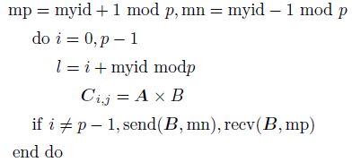
Combining parallel schemes to different portions,the framework of 3D parallel inversion algorithm in data space can be obtained,the flow chart of which is shown in Fig.2.

5 NUMERICAL EXPERIMENTS AND ANALYSIS OF PARALLEL PERFORMANCE

In order to test the effectiveness and efficiency of our 3D MT parallel inverse algorithm in data space,we generate synthetic data from two 3D models,and then use these synthetic data to test our algorithm on the Downing high-performance computing platform Dawn TC5000A.

5.1 Model I: 3D Prism Model

Model I is a 3D prism (Fig.3) consisting of a 1 Ωm prism body embedded into a 100 m half-space. The prism body has dimensions of 10 km×10 km×5 km and its top is 0.5 km below the earth’s surface. Twentyfive measurement sites are distributed uniformly on the earth’s surface. At each site,16 frequencies are computed (from 320 Hz to 0.005 Hz). Random errors with a relative magnitude of five percent of |Z_xyZ_yx|^1/2 are added to components of impedance data before inver-sion. The inversion model is discretized into 34×34×26 blocks,and all components of impedance data are involved into inversion. The desired misfit is set to 1,and the initial model is a 50 Ωm half-space.

The target misfit 0.98 is obtained after 6 iterations. Fig.4 demonstrates the inversion results of slices at different depths,and Fig.5 shows the inversion results of different sections. From Figs. 4 and 5,it can be noticed that the resolved resistivity images finely reflect the true shape and position of the anomalous body. Fig.6 displays the relationship between the number of iterations and data misfit RMS. From the first to the third iteration,the RMS decreases greatly and reaches the desired level of misfit at third iteration,which refers to the first stage of data-space approach; from the 4th to 6th iteration,the algorithm searches for the minimum structure model while keeping the data misfit at the desired level,which refers to the second stage of data-space approach.

5.2 Model II: 3D Complex Wedge Model

Model II is a 3D model with a 1 Ωm complex wedge,as shown in Fig.7. The measurement sites and frequencies as well as grid meshes are the same as model I. The initial model used for inversion is a 100 m uniform half-space. The inversion terminates after 10 iterations,and the final data RMS is 3.203. Fig.8 illustrates the inversion results of slices at different depths,and Fig.9 shows the inversion results of vertical section at x = 0. The true shape and position of anomalous body are well resolved (Figs. 8 and 9).

5.3 Analysis of Parallel Efficiency

In order to examine the parallel efficiency of 3D MT parallel algorithm in data space,we assign different numbers of computing nodes to invert synthetic data generated from model II. Two measures are defined to quantify the efficiency of the parallel algorithm. The first is parallel speedup which is the ratio of CPU times of serial algorithm to CPU times of parallel algorithm. The second measure is parallel efficiency which is the ratio of parallel speedup to the computing nodes. Table1 displays the statistical CPU time of serial and parallel inverse algorithm for model II.

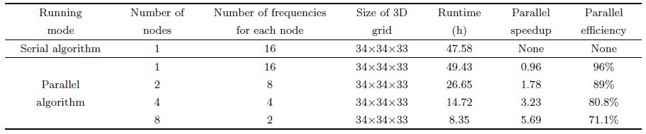
The parallel speedup increases with the increase of the number of computing nodes used for inversion. When the number of nodes is 4,the speedup could reach 3.23 and 5.69 for 8 nodes. As the time used for inversion decreases significantly,we can obtain the inversion images after relatively short time,which brings much convenience to 3D magnetotelluric inversion. Meanwhile,the parallel efficiency decreases gradually with the increase of the number of computing nodes. When 8 computing nodes are used in inversion,the parallel efficiency is merely 71.12%. This is because the increasing computing nodes require more time to pass messages between nodes. So controlling the amount of passing messages is crucial for the effectiveness of the parallel algorithm. In addition,it takes more time when using one computing node in the parallel algorithm than in the serial algorithm due to extra expense on message passing and data management. Overall,the parallel computing can significantly reduce the inversion time and meet the massive computation and memory requirement.

6 CONCLUSIONS

We implemented a 3D MT data-space parallel inversion algorithm using MPI on the Downing highperformance computing platform Dawn TC5000A. The parallel algorithm employs a coarse-grained parallelization scheme based on frequency division and matrix decomposition. This parallelization contains 3D forward modeling,sensitivity forming and matrix-vector multiplication as well as model update,which not just speeds up the calculation,but also reduces required memory. The numerical experiments for synthetic data from two models show that this 3D MT data-space parallel inverse algorithm is feasible and efficient. By assigning optimal computing nodes,we can obtain better parallel speedup and parallel efficiency. The parallel scheme provides a promising approach to the challenge of substantial computation and memory requirement in 3D MT inverse problems,which would advance the application of 3D MT inversion of field data.

7 ACKNOWLEDGMENTS

We thank Professor Weerachai Siripunvaraporn for providing original serial source codes for 3D magnetotelluric inversion. The implementation of parallel algorithm were on Downing high-performance computing platform Dawn TC5000A provided by China University of Geosciences,Wuhan. The clarity of this manuscript was improved by anonymous reviewers. This work was supported by the National Special Project of Deep Probing (SinoProb-01),the National Natural Science Foundation of China (40974040),and the Natural Science Foundation of Hubei Province (2011CDA123).