1 INTRODUCTION

Exploration seismology is an inversion problem in essence. The object of study is geophysical media. For the forward problem,the seismic wave propagation phenomenon is investigated. And for the inversion problem,the media parameters (velocity,density and anisotropy parameters) are estimated by back-propagating or projecting the acquired wave-fields (surface data,well log,cross-well,ocean bottom surface,etc.). The procedure of solving the geophysical parameters from seismic data is called seismic inversion. There are three levels of seismic inversion: geometrical structure description,amplitude preserved imaging and rock parameters estimation. Traditional migration imaging methods solve the problem of geometrical structure description^[1]. The purpose of seismic inversion is to solve the problem of rock parameters estimation^{[2, 3]}. For the second problem,amplitude preserved imaging,we need to combine the migration imaging and the inversion frame. From the point of view of imaging,the factors influencing the final imaging results include spherical spreading effect,surface consistency,accuracy of propagator and rock’s absorption and attenuation^[4]. Least-squares migration (LSM) estimates an optimized imaging result under the inversion frame^[5]. LSM can adjust most of the above factors during imaging via the Hessian operator^{[6, 7, 8]}. The Hessian operator includes all the information which can be described by the wave equation. It is difficult to solve the accurate Hessian operator and to invert. The same problem is present in the Gauss-Newton full waveform inversion (FWI) where the Hessian operator is used as a precondition to raise the inversion efficiency^[9]. In this paper,we present two new transformed Hessian forms which can be used into LSM and FWI. Numerical tests prove our method is effective in synthetic dataset processing.

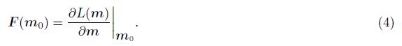
2 SEISMIC INVERSION AND HESSIAN OPERATOR

The seismic wave propagation and reception can be formulated as

where mtrue denotes the true seismic model parameters,like velocity,density,and elastic parameters,dobs is the observed seismic data,L(·) describes the system of seismic wave propagation. The seismic inversion can be formulated as where L^-1(·) denotes all the mathematical methods to project/propagate the observed data dobs to an estimated model mest. The seismic inversion problem is more complex than the forward problem. That is because the forward propagation just brings the information from the initial model. Seismic inversion complies the rule of the inversion problem summed up by Jacques H_adamard^[10]: (1) Existence. For given data d,there is a model m which satisfies d = L(m). (2) Uniqueness. There is only one m. (3) Stability. The perturbation data just reflects the perturbation model. If the inversion problem does not satisfy one of the three conditions,the problem is ill conditioned. Unfortunately,the conditions are usually not satisfied for seismic inversion. The reasons include the limited acquisition aperture,frequency band,and sparse sampling intervals. Also,the factors,which can not described by the wave equation,like the noise,can enlarge the ill condition.

2.1 Newton Inversion

In essence,seismic inversion is a nonlinear problem,i.e. the forward operator changes nonlinearly with model parameters. But for convenience,people often linearize the problem to calculate. To solve a inverse problem,a misfit function under the L2 norm is defined as

where the superscript T stands for the matrix transpose,and m is the parameter related to velocity in the acoustic media. Eq. (3) defines the basic least-squares misfit function. The Fr′echet derivative is

In the nonlinear problem,the Fr′echet derivative depends on the model. The Newton method assumes that the misfit function satisfies the quadratic form. Using the Taylor expansion:

where△_mE(m₀) = F _m0△d^T(m₀) is the value of the derivative of the misfit function near the initial model m₀,H is the second derivative of the misfit function to the model: where H is the so-called Hessian operator. The Hessian operator includes two parts. △d∂F^T/∂m is the nonlinear term and is related to the model. For the linear problem,the non-linear term equals to zero and we have

2.2 Mathematical and Physical Meanings of the Hessian Operator

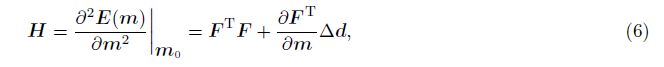
Mathematically,the Hessian operator is the second derivative of the misfit function to the model. In physics,we calculate the Hessian operator based on the wave equation to discuss its meaning. In the FWI,the exact Hessian operator includes two terms: linear term H_a and the nonlinear term R. In most cases,the computational amount is huge to calculate R. Under the assumption of local linearization,R approaches towards zero. So,we firstly need to study the approximateH_a which is also a difficult point in the Gauss-Newton FWI and the LSM.

Starting from the acoustic wave equation,there is

where f(x_s,ω) is the source wavelet in frequency domain excited from the shot point xs,and v(x) is the velocity of the media point. The wavefield varies with the media velocity. If we set v(x) as the inversion parameter,the gradient and Hessian term of the misfit function of Eq.(5) are From Eq.(10),we can see the exact Hessian H(x,y) is corresponding to two scattering points x and y. The nonlinear term R is the part behind the plus sign in Eq.(10).

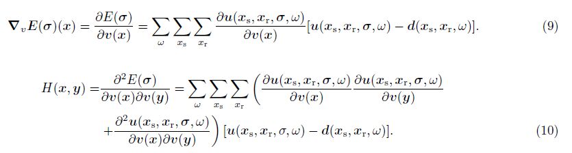
Under the Born approximation^[11] (local linearization),the seismic wavefield at the receiver point is

Combing Eqs.(8)-(11),we have The migration image can be viewed as a process of backward projecting the information from the seismic data to the model using a propagator. On the contrary,seismic modeling is a process of forward projecting the information from the model to the seismic data using a propagator. In the linear case under the Born approximation,there is where the propagator vector L which connects two fields and has two elements, The linearized Hessian matrix can be expressed as The corresponding gradient term is The general Newton inversion is The Linearized form which is so-called Gauss-Newton equation can be written as Suppose the a prior knowledge of the model m(0) = 0,the first iteration becomes

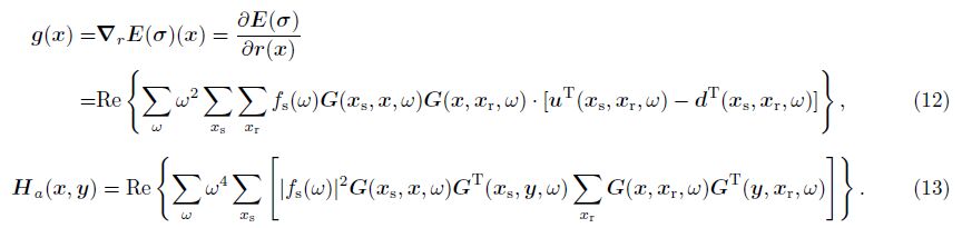
The gradient term L^Td in the first iteration stands for the seismic migration which back-propagates the data to image. Besides the Hessian operator H_a = L^TL,the migration imaging process can be seen as a half time iteration^[12],

In the frame of inversion,seismic modeling and migration can be explained in nature. In this paper’s mark,the forward modeling operator is L and its conjugate operator L^T stands for the migration operator. Based on the operators,the Hessian operator plays a role as precondition which can be used to the inversion imaging.

3 THE NATURE OF THE HESSIAN OPERATOR AND ITS APPROXIMATION

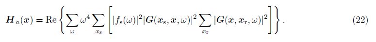
The Hessian operator takes a significant position in seismic inversion. But for both the Gauss-Newton FWI and LSM,a serious problem caused by the Hessian operator is its huge scale (elements of squared model parameter number). To avoid the difficult of solving and inverting the Hessian operator,many approximation forms have been proposed to replace the exact one. Yu et al.^[13] presented an inversed Hessian scheme in a v(z) medium. Lecomte^[14] solved the inversion problem based on the ray theory. Plessix and Mulder^[5] derived the Hessian matrix in the space domain and suggested four approximation forms for the diagonal Hessian. Tang^[15] used the phase-encoding method to calculate the Hessian matrix in a fast way. From the previous study^[7],the linearized Hessian matrix is a main diagonal dominant banding one. Using the diagonal elements of the Hessian matrix which is commonly so-called pseudo-Hessian,traditional Gauss-Newton inversion is realized. This pseudo-Hessian is expressed as

Eq.(22) is a matrix which spreads in the model space. The matrix reflects illumination to the subsurface from both the source and receiver points.

3.1 Planewave Hessian Operator and LSM

The LSM can remove the effects caused by acquisition aperture,footprint,and absorption attenuation. Meanwhile the LSM equation based on the inversion frame can be used to different operators. If only a suiTable forward modeling operator L and its adjoint migration operator L^T are estimated,the gradient term and Hessian can be calculated by the matrix operation.

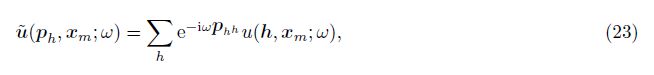
Offset continuation is one of the seismic data projection methods. Bagaini^[16] derived the offset continuation form in the shot domain. Formel^[17] modified the equation and presented a more precise one. Based on this thought,the shot domain wavefield can be decomposed into the planewaves:

where x_m is the common middle point (CMP),h is the offset,and p_h is the offset planewave ray parameter. Eq.(23) expresses the process of transforming a single frequency ω data u(h,x_m; ω) into planewave data u (p_h,x_m; ω) which corresponds to the CMP and ray parameter.

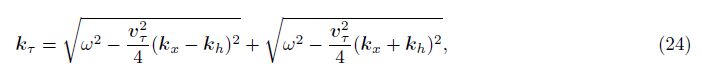
The double square root (DSR) operator for prestack time migration (PSTM) in the frequency-wavenumber domain can be expressed as

where k_x and k_h are the wavenumber corresponding to the CMP x_m and the offset h, τ is the time-depth for the PSTM,and v_τ and k_τ are the velocity and wavenumber separately corresponding to τ which is uncorrelated to x_m under the assumption of horizontal invariance. Eq.(24) can be rewritten as From Stolt and Benson^[18],we have tanθ = -v_τk_h/(2k_τ). The angle θ is between the incident direction and the reflect direction. So we have the relation The DSR operator can be written further The relation between the ray parameter and the angle is So the frequency-offset ray parameter domain wave equation becomes Eq.(29) can be solved by the finite difference method. The full image is the stack of images with different ray parameters The LSM needs firstly to estimate a migration operator. From Eqs.(23) to (30),the migration operator can be expressed as Next we calculate the migration operator L^*(τ,p_h; ω). If we construct a virtual source v(p_h,y_m; ω) and the elements number of p_h and y_m are equal,the seismic data matrix v(p_h,y_m; ω) is main diagonal dominance. In this case,the imaging result p(τ,y_m; ω) from Eq.(30) equals to the migration operator L^*(τ,p_h; ω). The migration operator can be calculated in the time domain by the finite difference method^[19]. After generating the migration operator,the forward modeling operator L(p_h, τ; ω) can be calculated by the complex conjugation. The planewave PSTM domain Hessian matrix can be calculated by It is clear that the transform Hessian operator in the planewave domain reflects the relation between different ray parameters. When p_h = p_h' ,the diagonal Hessian Hz(p_h) reflects the illumination energy of different ray parameters. The corresponding LSM form can be carried out naturally.

3.2 Offset Hessian Operator and Newton FWI

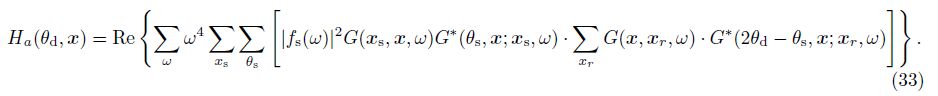
Under the traditional Newton FWI frame,the Hessian operator is used as a preconditioner to increase the iteration efficiency. But how to estimate a corresponding Hessian is difficult. In the early study,we developed a local angle domain Hessian operator^[7] which matches the wavelet domain propagator. The local angle domain Hessian operator is corresponding to the imaging points x and the dip-angle

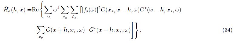
This transformed Hessian operator can be applied to the LSM but can not be used to FWI easily. Here,we propose a new similar sub offset domain Hessian form

Since the new form does not need to do the angle decomposition after full wave propagation,it can be used to the sub offset common image gathers using the expanded imaging condition^{[20, 21]}. We expect it can increase the inversion efficiency. For convenience,we also can move the two Green’s functions corresponding to the receiver point and just use the shot domain illumination.

4 NUMERICAL TESTS 4.1 Planewave LSM

Firstly,we test the planwave Hessian using a simple model. On the model shown in Fig.1a,5 shots dataset are synthesized from the star-marked points with the main frequency of 30 Hz. Two reference traces are chosen to test the planewave domain Hessian and LSM. Fig.1b and 1c give the direct planewave migration results and the planewave LSM results using the planewave Hessian shown in Fig.1d. It is apparent that the LSM results are better both in the resolution and illumination. For this model,the planewave Hessian is main diagonal dominance. Fig.1e and 1f show the reflectivity,direct imaging results and LSM imaging results for two reference traces marked in Fig.1a,respectively. Comparison indicates that the LSM result has better resolution and balanceed illumination than the direct one.

4.2 Quasi-Newton Inversion Based on Subsurface Offset Hessian

The Full Waveform Inversion (FWI) has the highest resolution theoretically. But the expensive computation is a great challenge for FWI. We use the transformed Hessian operator in Eq.(34) as a preconditioner for the quasi-Newton FWI and apply it to the Marmousi model. Starting from a smoothed initial model (shown in Fig.2a),we perform the general conjugate gradient (CG) FWI,shot illumination preconditioned FWI and the Offset Hessian preconditioned FWI (Fig.2(b-e)). From the convergence curve shown in Fig.2f,after the preconditioner of both shot illumination and offset Hessian is used,the convergence is significantly faster than the traditional CG method. Although the stability of full sub offset Hessian preconditioned FWI needs to be studied further,the general convergence trend with this method is acceptable.

5 CONCLUSIONS AND DISCUSSION

Starting from the Newton inversion frame,this paper discusses and analyzes the Hessian operator in seismic inversion imaging both mathematically and physically. In math,the Hessian operator is the second derivative of the misfit function to the model. So,whether the variation of misfit function with respect to the model satisfies the quadratic form is a problem. Previous studies pointed out that the seismic inverse problem is strongly nonlinear. But we can assume that in a local area,the problem is quadratic or even linear. This approximation can be utilized in the Born assumption which can lead to the LSM and FWI. So,the methods we proposed in this paper also need a good initial macro velocity model. Under the acoustic equation,the Hessian matrix can be expressed as the Green’s function. An exact invert Hessian operator can generate an amplitude-preserved result. The planewave Hessian proves the capability of the LSM. Similarly,the Newton inversion based on the quadratic assumption can produce a better result. The subsuface offset Hessian applied to FWI can result in a fast convergence. In sum,the Hessian operator has a significant value in seismic inversion imaging. The study on further enhancement of calculation efficiency and stability will be the next target in the future.

ACKNOWLEDGMENTS

The authors thank the financial supports by SINOPEC Key Laboratory of Geophysics Foundation,Zhejiang Province Postdoc Preferential Foundation (Bsh1202046) and National Natural Science Foundation of China (NSFC) (ID: 41304089). The first author was grateful to the Wave Phenomenon and Inversion Imaging (WPI) research group at Tongji University for the discussions and suggestions.