 2013, Vol. 56


2. State Key Laboratory of Geodesy and Earth Geodynamics, Institute of Geodesy and Geophysics, Chinese Academy of Sciences, Wuhan 430077, China;
3. School of Earth Sciences, University of Chinese Academy of Sciences, Beijing 100049, China
Teleseismic body wave receiver function is widely applied to study the earth inner structure since the 1980s. Teleseismic body wave receiver function is related to inferior medium structure beneath seismic station,it has nothing to do with hypocenter and travel path by theory and experiment research. So it is an important method to study crustal and upper mantle velocity structures and discontinuity surface fluctuation characteristics by teleseismic body wave receiver function data in recent years[1, 2, 3, 4, 5]. The studies about broadband seismograph receiver function have done quite a lot of work and got many solutions. Some researchers have done a few applying short-period seismograph receiver functions,but research on stability and reliability of short-period seismograph receiver function is rare[6, 7, 8, 9, 10, 11]. Regional digital seismic network built in 1999-2001 in 20 provinces includes 381 seismic stations,short-period seismographs with a dynamic range less than 90 dB are equipped at about 320 seismic stations[12]. Now a large number of short-period seismographs exist nationwide in regional and local digital seismic networks,there are 150 short-period seismographs in nationwide regional stations,and a great deal of short-period seismographs exist at mobile seismic networks of seismic field emergency and earthquake science exploration arrays[13, 14]. Lots of teleseismic waveform data are recorded in long-term by short-period seismographs. A lot of short-period seismographs are located in the area where the broadband seismograph is rare,for example,in Capital Area network,a large portion of teleseismic waveform data are recorded by short-period seismographs. If we can utilize short-period teleseismic waveform data sufficiently,combine long-period and short-period data,and explore the method that uses short-period data to research receiver function,it will increase the number of data,attain more accurate understanding of crustal structure,and offer more reliable foundation to study of seismic activity and seismogenic structure.
Stability and reliability of result must be analysed when studying receiver function by short-period seismograph data. For understanding and estimating feasibility quantitatively,a feasible scheme is to comparatively analyze the broadband and short-period seismograph waveform data at the same seismic station. Xinjiang Hotan Seismic Array was built in 2007 with an aperture about 3 km,including 9 sub-stations,same type shortperiod three-component seismographs were installed in every sub-station,a very broadband seismograph was installed at the central station (sub-stations 1). Ideal foundation is provided to study short-period seismograph receiver function by Hotan Seismic Array. This paper probes the feasibility of short-period seismograph receiver function,quantitatively analyzes the stability and reliability of short-period seismograph receiver function,and investigates crustal thickness,Poisson’s ratio and S wave velocity structure beneath Hotan Seismic Array based on 3 years waveform data recorded by Hotan Seismic Array. The paper provides quantitative evidence to shortperiod seismograph receiver function application for using the same method to study the structure in other areas of Xinjiang.
2 GENERAL SITUATION OF XINJIANG HOTAN SEISMIC ARRAYHotan Seismic Array is located at the Piyaman Anticline,Pishan County,Hotan of Xinjiang in the junction zone of southwest Tarim Basin and the West Kunlun Mountains. The elevation of Hotan Seismic Array is between 1580 m and 1650 m,relative height difference less than 80 m. Most stratums belong to Permian sand-stone,some place is limestone and mudstone at Hotan Seismic Array. The configuration of Hotan Seismic Array is annular,with sub-stations at concentric circles,and the aperture diameter is about 3 km. The inner circle includes 3 sub-stations,aperture is 600 m,outer circle includes 5 sub-stations,aperture is about 1500 m. The distribution and distance of sub-station to central station is seen in Fig.1. Same type short-period three-component seismograph is equipped at every sub-station (type: CMG-40T-1,frequency bandwidth is about 2 s~40 Hz). On the same seismic pendulum mound of central sub-station (below called as sub-station one or TZ1) a very broadband seismograph was installed. The data acquisition unit is EDSP-24IP,sampling frequency is 100 Hz.

|
Fig.1 Configuration of Hotan Seismic Array |
Time domain iteration deconvolution method is adopted to calculate receiver function[15]. The method is used to solve radial component receiver function ER(t),that is to find the minimum value of equation 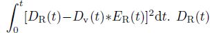 is the radial component of teleseismic wave,Dv(t) is the vertical component. Dv(t)*ER(t) is the convolution of the updated receiver function from recent iteration and the vertical component of observed seismogram. The goodness of receiver function can be judged by the fitting coefficient of Dv(t)*ER(t) and DR(t).
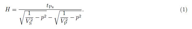
For an one-dimensional horizontal single-layer crustal model,when the P wave and S wave average crustal velocity VP and VS are given,crustal thickness H can be obtained by formula (1),tPs is the arrival time difference between Ps and first arrival P,p is the ray parameter of incident P wave

After gaining single station receiver function,the S-wave velocity structure beneath the station can be achieved by receiver function wave inversion. Owens et al. developed a time domain inversion technology,it can invert for the one-dimensional velocity structure beneath single station from receiver function[20, 21, 22]. By seismic wave propagation matrix theory of layered elastic medium,we can calculate and obtain the theoretic receiver function of layered medium and the partial derivatives to every layer elastic parameter,the one-dimensional velocity structure beneath the station can be obtained from receiver function by iterative linear inversion.
4 ANALYSIS AND DISCUSSION 4.1 Comparison and Analysis of Hotan Seismic Array Receiver Function 4.1.1 Receiver function calculation of Hotan Seismic ArrayWe select 596 teleseismic waveforms with magnitude M ≥λ 5.5 and epicentral distance between 30° ~ 90° recorded by Hotan Seismic Array,the distribution of earthquakes is shown in Fig.2. The receiver function of each station is calculated,and those with fitting coefficients greater than or equal to 0.95 are selected for analysis. Receiver functions contain some high-frequency noise because of influence of recording noise,interface small scale fluctuation,anisotropy and heterogeneous body volume scattering and so on,which is generally suppressed by Gaussian low-pass filtering. For teleseismic receiver functions the Gaussian filter factor α is 1.5 or 2.5 normally. For determining the common frequency range of short-period and broadband receiver functions,Fig.3 shows the amplitude-response curves of shortperiod and broadband seismographs Gaussian filters with different factors used in this paper. Set the frequency corresponding to amplitude value 0.1 as the cut-off frequency,broadband receiver function contains more low frequency information,short-period receiver function lacks information below 0.155 Hz. When α is 1.5,the common frequency range is from 0.155 to 0.725 Hz for both short-period and broadband receiver functions,when α is 2.5,the frequency range is from 0.155 to 1.208 Hz. With the increase of Gaussian filtering factor α,the common frequency band is broader,there is more noise signal in receiver function too. For understanding the influence of different α value on short-period seismograph receiver function,we set α as 1.5 and 2.5 respectively,obtain the receiver functions in different frequency bands,then analyze the influence of α value on the stability of short-period seismograph receiver functions.

|
Fig.2 Distribution of teleseismic events used in this study Circles are the teleseismic earthquakes,the triangle shows the location of Hotan Seismic Array. |

|
Fig.3 Amplitude response curve The red line is broadband seismometer amplitude response curve,the blue line is the short-period seismometer amplitude response curve,the black line is amplitude response curve of Gaussian filter with different coefficient value; the red circle indicates the frequency when short-period seismograph amplitude response value is 0.1,the red star is the frequency when Gaussian filter amplitude response value is 0.1. |
To improve signal-to-noise ratio,we stack receiver functions of each station separately. The incident angle is different for teleseismic body waves with different ray parameters,which affects the receiver function amplitude and arrival time. For comparing the receiver function waveforms and amplitudes obtained by shortperiod and broadband seismographs,and eliminating the effect caused by different ray parameters,we select receiver functions with ray parameter difference less than 0.01 s/km in stacking and averaging,obtain the stacked receiver functions of different ray parameters for 9 short-period stations of Hotan Seismic Array and broadband seismograph receiver functions. To quantitatively analyze the stability and reliability of shortperiod seismograph receiver function,we calculated the correlation coefficients and amplitude differences of short-period and broadband seismograph receiver functions with different ray parameter. When calculating the correlation coefficient of receiver functions,the time window length is from 1 second before to 40 seconds behind the 0 moment,which includes the seismic phases such as the first arrival P-wave,Moho Ps converted wave and multiple reflection converted waves in the receiver function.
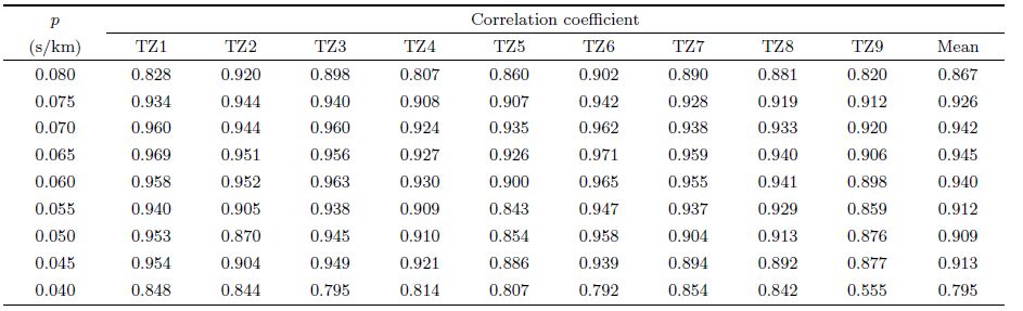
Table1 and Table2 are the receiver function correlation coefficients of Hotan Seismic Array short-period sub-station and sub-station 1 broadband seismograph. As an example,Fig.4 shows the receiver functions of sub-station 1 short-period and broadband seismograph when α is 1.5 and 2.5.

|
Fig.4 Comparative analysis of teleseismic receiver function waveform between short-period and broadband seismograph of TZ1 in Hotan Seismic Array (α = 1.5 (a),α=2.5 (b)) The red waveforms are receiver functions of broadband seismograph,the grey areas are receiver functions stack standard deviation of TZ1,the blue waveforms are short-period seismograph receiver functions of TZ1,the numbers on the left of receiver functions are the stack receiver functions number. |
| Table 1 Correlation coefficients of teleseismic receiver function waveform between 9 short-period and substation-one broadband seismographs of Hotan Seismic Array (α = 1.5),p is the ray parameter |
| Table 2 Correlation coefficients of teleseismic receiver function waveform between 9 short-period and substation-one broadband seismographs of Hotan Seismic Array (α = 2.5),p is the ray parameter |
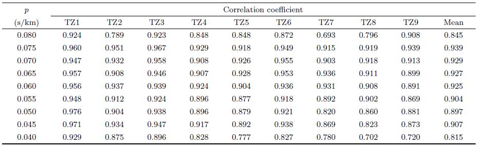
Figure4 shows that the first arrival seismic phase of Hotan Seismic Array receiver functions is sharp and the sediment beneath Hotan Seismic Array is very thin. Moho Ps converted phase is prominent,Ps wave arrival time is about 6.5 s later than the first arrival P-wave.
Table1 , 2 and Fig.4 indicate that the main seismic phases of short-period and broadband receiver functions accord well with each other in terms of arrival time and relative amplitude,no matter α is 1.5 or 2.5. The short-period receiver functions of 9 stations of Hotan Seismic Array have good linear correlation with the broadband receiver function of sub-station 1; except for the correlation coefficient less than 0.87 of receiver functions with ray parameter 0.04 s/km and 0.08 s/km,all others approach or exceed 0.9. The following analysis indicates that the lower correlation coefficient is related to the number and azimuth of receiver functions used in stacking. When α is 2.5,the correlation coefficient is maximum at TZ1. When α is 1.5,the high-frequency noise of receiver function decreases,but the correlation coefficient of short-period and broadband receiver functions at TZ1 is less than that when α is 2.5. By analysing the numbers and back azimuths (baz) of receiver functions used in stacking of each substation with different ray parameter,we find that for ray parameter between 0.060~0.075 s/km the average receiver functions consist of 12 or more receiver functions,and the azimuths concentrate in 96° ~ 118°. The average receiver functions with ray parameter 0.040 s/km or 0.080 s/km consist of 1~5 receiver functions respectively,and the direction of most single short-period receiver function is different from broadband receiver function (difference about 90°). We think that the smaller correlation coefficient of some ray parameters is caused by teleseismic wave sampling at different azimuths in the boundary area between the basin and the mountain where the structure changes markedly.
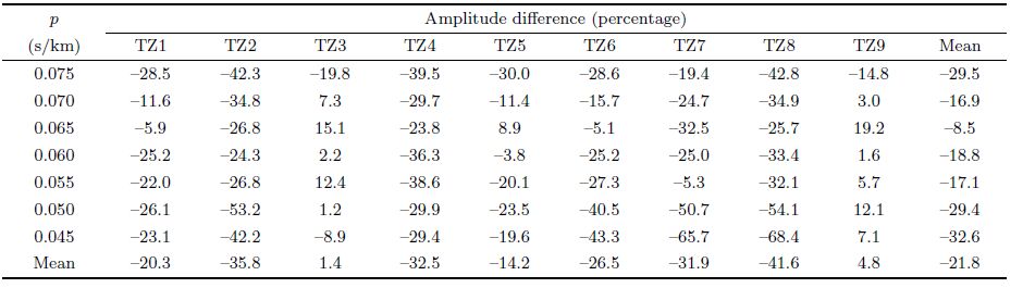
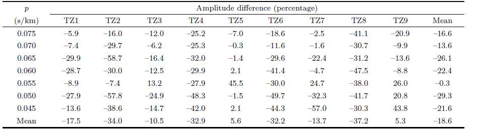
Because the amplitude of each receiver function phase is related to the velocity discontinuity across the interface[20, 23, 24, 25, 26],we can know the velocity change from the amplitudes of various phases of receiver function,and restrain the interface undulation and velocity change values. So by analyzing the amplitudes of short-period seismograph receiver functions,we can estimate their sensitivities to velocity interface. Aiming at the most clear Moho converted wave Ps,we compare and analyze Ps average single-point amplitude ratio Adiff of short-period and broadband seismograph receiver functions
Adiff = (As - Ab)/Ab × 100%,
As is the average amplitude of short-period seismograph stacked receiver function,Ab is the average amplitude of broadband seismograph stacked receiver function. It is seen from Table3 and 4 that,when α is 2.5,the average amplitude difference of short-period and broadband receiver function Ps phase at the central sub-station TZ1 is -17.5%,which is less than the amplitude difference -20.3% when α is 1.5. Comparing the amplitude responses of short-period and broadband seismographs (Fig.3),under 1 Hz frequency,the amplitude response of short-period becomes less than broadband gradually. With the decrease of Gaussian filter factor,the center frequency of short-period receiver function decreases,the amplitude value deviates from broadband receiver function amplitude severely. We think that the amplitude of short-period receiver function is smaller than that of broadband,and with the decrease of Gaussian filter factor,the degree of deviation is serious. This is because that the amplitude response of short-period seismograph is less than broadband seismograph in this signal frequency range.
| Table 3 Amplitude difference of teleseismic receiver function Ps phase between 9 short-period and substation-one broadband seismographs of Hotan Seismic Array (α = 1.5),p is the ray parameter |
| Table 4 Amplitude difference of teleseismic receiver function Ps phase between 9 short-period and substation-one broadband seismographs of Hotan Seismic Array (α = 2.5),p is the ray parameter |
By comparison and analysis,the following results are obtained. (1) Short-period seismograph can produce reliable teleseismic receiver function,the waveform and arrival time of receiver function are highly consistent with broadband seismograph,when α is 2.5,the short-period seismograph receiver function is closer to broadband seismograph receiver function. (2) Due to the restriction of short-period seismograph frequency range,Gaussian filter factor α affects the amplitude of short-period receiver function severely,to restrain high-frequency noise,small Gaussian filter factor is selected,and the amplitude difference of short-period and broadband seismograph receiver function will increase. So we estimate that short-period seismograph can replace broadband seismograph successfully when studying the crustal structure by receiver function seismic phase arrival times. Short-period seismograph receiver function will underestimate the velocity change at interface when using receiver function waveform inversion for the velocity structure beneath seismic station.
4.2 Crustal Thickness and VP/VS Beneath Hotan Seismic Array by Short-Period SeismographReceiver Function H-κ grid-stacking-search method uses the first and multiple converted waves of receiver function arrival time information to obtain regional crustal average thickness and VP/VS. We can check the stability and reliability of applying short-period seismograph receiver function to study crustal structure. For different α values,we carried out H-κ processing of the selected individual and epicentral distance-stacked receiver functions respectively for each sub-station of Hotan Seismic Array. In the H-κ stacking,all parameter values are the same. Referring to available geophysical research result in the areas adjacent to Hotan Seismic Array[27, 28, 29, 30, 31],we set the average crustal P-wave velocity as 6.0 km/s.
Table5 is the crustal thickness and VP/VS obtained by H-κ grid-stacking-search method. "H1" and "≤1" are crustal thickness and VP/VS obtained from selected individual receiver functions of each sub-station. "H2" and "κ2" are crustal thickness and VP/VS obtained from epicentral distance-stacked receiver functions of each sub-station. Table5 also shows the number of receiver functions used in H-κ grid-stacking for different α values. It manifests that the result of crustal thickness is consistent from either broadband or short-period seismograph receiver functions under all conditions,the average value is 54 km.
| Table 5 Crustal parameters obtained by H-κ grid-stacking-search method at each station of Hotan Seismic Array |
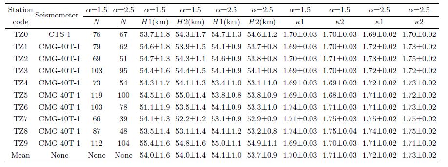
From Table5 we know that the crustal thickness beneath Hotan Seismic Array is 54.0 km,average VP/VS is 1.71 (Poisson’s ratio is 0.24). This value coincides with the former result (about 55 km) by seismic exploration[27, 28, 29, 30, 31],deep seismic reflection and broadband seismic exploration in southwest Tarim and West Kunlun Mountains contact zone. It is also consistent with the crustal thickness (51.81 km) and Poisson’s ratio (0.258) obtained by Chen et al.[32] by receiver function method. Whether α is 1.5 or 2.5,it is reliable to study Moho depth and average VP/VS by short-period seismograph receiver function.
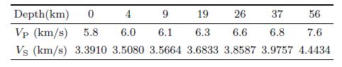
4.3 S-wave Velocity Structure Beneath TZ1 of Hotan Seismic Array 4.3.1 Initial velocity modelReferring to previous geophysical research results in the Tarim and the east Kunlun Mountains contact zone[27, 28, 29, 30, 31],a P-wave velocity model is built as shown in Table6. The S-wave velocity is derived from the P-wave velocity divided by the average wave velocity ratio 1.71.
| Table 6 Initial model of velocity structure beneath Hotan Seismic Array |
To investigate the difference of velocity structures derived from broadband and short-period receiver functions,we adopt Herrmann and Russell time domain linear inversion method[33, 34, 35],utilize broadband and short-period receiver functions,and invert for the crustal S velocity structure beneath TZ1 (Fig.5). Wu et al.[36] manifested that joint inversion of receiver functions in different frequency range can reduce the dependence of generalized linear inversion on the initial model,eliminate waveform inversion non-uniqueness to some extent. So we use the average receiver functions with different ray parameters in the inversion at the same time. In view of the stability of receiver function stack,we select the average receiver functions with ray parameter between 0.060 and 0.075 to inversion.

|
Fig.5 The S wave velocity structure beneath TZ1 of Hotan Seismic Array The green line is initial model. The red line is the VS model from receiver function of broadband seismograph of TZ1. The blue line is the VS model from receiver function of short-period seismograph of TZ1. |
Comparing the velocity structure inversion results of broadband and short-period receiver functions,the following results are obtained. (1) When α is 1.5 and 2.5,the inversion result of TZ1 broadband seismograph receiver function is consistent,which indicates that the shallow layer has low velocity,in 2~10 km is high velocity layer,10~20 km is low velocity layer,20~40 km velocity variation is stable,large velocity variation happens at Moho. (2) When α is 1.5 and 2.5,in 4~20 km depth,S wave velocity from short-period receiver function inversion is a little more than that from broadband data (about 0.1 km/s larger); beneath 40 km,the S wave velocity from short-period receiver function inversion is about 0.3 km/s less than that from broadband data.
Due to the insensitivity of receiver function to velocity value,the existence of record noise,and strong non-uniqueness in receiver function inversion,we think that the velocity deviation of 0.1 km/s in the upper-middle crust is within the error range. The crustal structure from broadband receiver function indicates that middle-lower crustal velocity transition is stable,but inversion result of short-period receiver function displays a low velocity zone in middle-lower crustal. The two kinds of distinct crustal model will produce prominent influence to geological evolution and dynamics process. We think that the wave velocity deviation as high as 0.3 km/s in the lower crust is mainly because the waveform amplitude of short-period receiver function from lower crust and Moho interface is generally less than that of broadband receiver function (Table3,Table4,Fig.4). Because the short-period seismogram lacks low-frequency signal under 0.155 Hz,the attenuation of low-frequency signal is slow with increasing distance,so with the increase of inversion depth,low-frequency signal energy proportion in all waveform is enhanced gradually. On the other hand,the amplitude response of short-period seismograph is below that of broadband seismograph in usual receiver function frequency range,and exhibits a non-linear relationship with frequency decrease,so it should be more careful using short-period receiver function waveforms to obtain inversion velocity structure and make interpretation. Combining other data sensitive to wave velocity,for example surface wave dispersion curve,with short-period receiver function in joint inversion[37] will contribute to enhance the reliability of velocity structure.
5 CONCLUSIONS AND UNDERSTANDINGThis paper evaluates the reliability and feasibility of utilizing short-period seismograph receiver functions by analyzing the receiver function correlation coefficient and amplitude difference between 9 short-period substations of Hotan Seismic Array and sub-station 1 broadband receiver functions,and crustal thickness,VP/VS and S-wave velocity structure beneath TZ1. Some conclusions are obtained.
(1) The high quality receiver function can be obtained by short-period seismograph. Whether the Gaussian coefficient value is 1.5 or 2.5,very good linear correlation (correlation coefficient is about 0.9) exists between the receiver function waveforms (leading 41 s) of 9 short-period sub-stations and TZ1 broadband seismograph of Hotan Seismic Array,but there is a small amplitude difference (about 20%) of the converted wave Ps seismic phase. It manifests that fine receiver function can be obtained by short-period seismograph,it consists with the broadband seismograph receiver function.
(2) The value of Gaussian filter factor will affect the receiver function derived from short-period seismograms. When α is 2.5,the correlation coefficient of short-period and broadband seismograph receiver functions of sub-station 1 is greater than that when α is 1.5,and the amplitude difference of Ps phase is less than that when α is 1.5. When calculating short-period seismograph receiver function,taking greater Gaussian filter factor may reduce the difference with broadband receiver function,but more noise will be included. So we must select suitable method according to the purpose of research.
(3) When α is 1.5 or 2.5,the H-κ stacking-search-method results are consistent from 9 short-period substations and broadband seismograph of Hotan Seismic Array,the crustal thickness beneath Hotan Seismic Array is 54.0 km,crustal average Poisson’s ratio is 0.24. The short-period seismograph receiver functions can replace broadband seismograph receiver functions,if a method using the seismic phase arrival time of receiver functions is adopted (such as grid-stacking-search method).
(4) We notice that there are some differences in the crustal S-wave velocity structures obtained from short-period and broadband receiver functions,it is more obvious especially from lower crust to upper mantle top. The wave velocity value from lower crust to upper mantle top obtained by short-period receiver function inversion is a little smaller (about 0.3 km/s),but it possesses strong restraint on Moho interface position and velocity change features. So additional data sensitive to S-wave velocity structure value (such as surface wave dispersion) are needed for joint analysis.
ACKNOWLEDGMENTSWe are thankful to two anonymous experts for their constructive comments to improve the manuscript. This study is supported by the National Natural Science Foundation of China (41104037 and 41174086),the earthquake nonprofit industry special (201308013),the China Earthquake Administration,seismic networks young cadres training special (20130216) and Xinjiang earthquake science fund project (201103).
| [1] Teng J W, Zhang Z J, Bai W M, et al. Lithospheric Geological (in Chinese). Beijing:Science Press, 2004. |
| [2] Xu W W, Zheng T Y. The receiver function method and its progress. Progress in Geophysics (in Chinese), 2002, 17(4):605-613. |
| [3] Xu Q, Zhao J M. A review of the receiver function method. Progress in Geophysics (in Chinese), 2008, 23(6):1709-1716. |
| [4] Langston C A. Structure under Mount Rainier, Washington, inferred from teleseismic body waves. J. Geophys. Res., 1979, 84(B9):4749-4762. |
| [5] Langston C A. Evidence for the subducting lithosphere under southern Vancouver Island and eastern Oregon from teleseismic P wave conversions. J. Geophys. Res., 1981, 86(B5):3857-3866. |
| [6] Wang J, Liu Q Y, Chen J H, et al. The crustal thickness and Poisson's ratio beneath the Capital Circle Region. Chinese J. Geophys. (in Chinese), 2009, 52(1):57-66. |
| [7] Wang C Y, Lou H, Yao Z X, et al. Crustal thicknesses and Poisson's ratios in Longmenshan mountains and adjacent regions. Quaternary Sciences (in Chinese), 2010, 30(4):652-662. |
| [8] Li Y H, Wu Q J, Tian X B, et al. Crustal structure in the Yunnan region determined by modeling receiver functions. Chinese J. Geophys. (in Chinese), 2009, 52(1):67-80. |
| [9] Song W J, Zhu J S, Cheng X Q, et al. Deep crustal structure around the source area of the Wenchuan Ms8.0 earthquake. Quaternary Sciences (in Chinese), 2010, 30(4):670-677. |
| [10] Luo Y, Chong J J, Ni S D, et al. Moho depth and sedimentary thickness in Capital region. Chinese J. Geophys. (in Chinese), 2008, 51(4):1135-1145. |
| [11] He C S, Zhu L P, Ding Z F, et al. Sedimentary cover in the Bohai basin using teleseismic receiver function. Acta Geologica Sinica (in Chinese), 2010, 84(5):716-721. |
| [12] Liu R F,Wu Z L, Yin C M, et al. Development of China digital seismological observational systems. Acta Seismologica Sinica (in Chinese), 2003, 25(5):535-540. |
| [13] Liu R F, Gao J C, Chen Y T, et al. Construction and development of digital seismograph networks in China. Acta Seismologica Sinica (in Chinese), 2008, 30(5):533-539. |
| [14] Zheng X F, Ouyang B, Zhang D N, et al. Technical system construction of Data Backup Centre for China Seismograph Network and the data support to researches on the Wenchuan earthquake. Chinese J. Geophys. (in Chinese), 2009, 52(5):1412-1417. |
| [15] Ligorría J P, Ammon C J. Iterative deconvolution and receiver-function estimation. Bull. Seism. Soc. Am., 1999, 89(5):1395-1400. |
| [16] Zandt G, Myers S C, Wallace T C. Crust and mantle structure across the Basin and Range-Colorado Plateau boundary at 37°N latitude and implications for Cenozoic extensional mechanism. J. Geophys. Res., 1995, 100(B6):10529-10548. |
| [17] Zandt G, Ammon C J. Continental crust composition constrained by measurements of crustal Poisson's ratio. Nature, 1995, 374(6518):152-154. |
| [18] Zhu L P, Kanamori H. Moho depth variation in Southern California from teleseismic receiver functions. J. Geophys. Res., 2000, 105(B2):2969-2980. |
| [19] Li S B. Earthquake China (in Chinese). Beijing:Seismological Press, 1981. |
| [20] Owens T J, Taylor S R, Zandt G. Crustal structure at regional seismic test network stations determined from inversion of broadband teleseismic P waveforms. Bull. Seism. Soc. Am., 1987, 77(2):631-632. |
| [21] Owens T J, Zandat G, Taylor S R. Seismic evidence for an ancient rift beneath the Cumberland Plateau, Tennessee:A detailed analysis of broadband teleseismic P waveforms. J. Geophys. Res., 1984, 89(B9):7783-7795. |
| [22] Owens T J, Crosson R S. Shallow structure effects on broadband teleseismic P waveforms. Bull. Seism. Soc. Am., 1988, 78(1):96-108. |
| [23] http://eqseis.geosc.psu.edu/-cammon/HTML/RftnDocs/rftn01-06.html. |
| [24] Wu Q J, Li Y H, Zhang R P, et al. Receiver functions from autoregressive deconvolution. Pure and Applied Geophysics, 2007, 164(11):2175-2192. |
| [25] Burdick L J, Langston C A. Modeling crustal structure through the use of converted phases in teleseismic body waveforms. Bull. Seism. Soc. Am., 1977, 67(3):677-691. |
| [26] Ammon C J. The isolation of receiver effects from teleseismic P waveforms. Bull. Seism. Soc. Am., 1991, 81(6):2504-2510. |
| [27] He R Z, Gao R, Li Q S, et al. Corridor gravity fields and crustal density structures in Tianshan (Dushanzi)-west Kunlun (Quanshuigou) GGT. Acta Geoscientia Sinica (in Chinese), 2001, 22(6):553-558. |
| [28] Gao R, Xiao X C, Gao H, et al. Summary of deep seismic probing of the lithospheric structure across the West Kunlun-Tarim-Tianshan. Geological Bulletin of China (in Chinese), 2002, 21(1):11-18. |
| [29] Li Q S, Lu D Y, Gao R, et al. Explosion seismic probing across the West Kunlun-Tarim contact zone. Science in China (Series D) (in Chinese), 2000, 30(B12):16-21. |
| [30] Gao R, Guan Y, He R Z, et al. The integrated geophysical observation and research along the Xinjiang (XUAR) geotransect and its surrounding areas. Acta Geoscientia Sinica (in Chinese), 2001, 22(6):527-533. |
| [31] Gao R, Xiao X C, Liu X, et al. Detail lithospheric structure of the contact zone of west Kunlun and Tarim revealed by deep seismic reflection profile along the Xinjiang geotransect. Acta Geoscientia Sinica (in Chinese), 2001, 22(6):547-552. |
| [32] Chen Y L, Niu F L, Liu R F, et al. Crustal structure beneath China from receiver function analysis. J. Geophys. Res., 2010, 115:B03307, doi:10.1029/2009JB006386. |
| [33] Ammon C J, Randall G E, Zandt G. On the nonuniqueness of receiver function inversions. J. Geophys. Res., 1990, 95(B10):15303-15318. |
| [34] Randall G E. Efficient calculation of differential seismograms for lithospheric receiver functions. Geophys. J. Int., 1989, 99(3):469-481. |
| [35] http://www.eas.slu.edu/People/RBHerrmann/ComputerPrograms.Html |
| [36] Wu Q J, Li Y H, Zhang R Q, et al. Wavelet modelling of broad-band receiver functions. Geophys. J. Int., 2007, 170(2):534-544. |
| [37] Shen W, Ritzwoller M H, Schulte-Pelkum V, et al. Joint inversion of surface wave dispersion and receiver functions:A Bayesian Monte-Carlo approach. Geophys. J. Int., 2013, 192(2):807-836. |