 2013, Vol. 56


Earthquakes are one of the most destructive natural disasters which can cause huge losses of people’s life and economy. To reduce hazards of earthquakes,a lot of efforts have been made to explore new approaches to predict earthquakes. Of them,the study on ionospheric disturbance during major earthquakes has received much attention[1, 2, 3, 4]. In 1964,Barnes et al.[5] reported such a phenomenon associated with the Alaska great earthquake. Since then,many researchers have studied the relationship between ionospheric changes and earthquakes,which were expected to be used in short-term prediction. Statistics shows that there exist anomalies of total electric content (TEC) in the ionosphere over the earthquake epicenter and adjacent areas,TEC obviously reduced within 10 days before a major earthquake[6, 7, 8, 9, 10, 11, 12]. Liu et al.[11] analyzed critical frequency variations of the F2 layer in the ionosphere before M6 events around Taiwan during 1994-1999. They noted that TEC at local time 12:00-17:00 1~6 days before the earthquakes decreased remarkably relative to their mean values 15 days ago,and regarded it as a seismic precursor. Based on review to studies of 10 years on this subject,Pulinets et al.[12] described the features of ionospheric disturbance before earthquakes. Meng et al.[8] found that TEC of the ionosphere became small 1~4 days prior to earthquakes,and TEC values were all lower than that of quiet time. Zhu et al.[13] used the sliding window and Inter Quartile Range methods to analyze ionospheric disturbance before the Wenchuan earthquake,and found TEC anomalies tended to shift toward the equator. And Yao et al.[14] employed the sliding window method to analyze the data of M7 earthquakes of 2010 in the world,and thought that ionospheric disturbance did not always occur before these events,no unified rules.
In detection of pre-seismic anomalies in the ionosphere,whether its results are accurate depends on the precision of reference background values and their upper and lower limits. Current methods in this field,such as the average,medium value,Inter Quartile Range,and sliding window,only consider their definite components,while the uncertainty is ignored. Thus the accuracy in prediction of TEC background values is relatively low. Besides,these methods lack of reasonable unified standards to determine upper and lower limits of reference background values,and are easy to cause errors in detection and bring about serious effects on subsequent results.
To solve this problem,this paper proposes a time series method based on the Autoregressive Integrated Moving Average (ARIMA) model. First,we compare the accuracies of this new method and conventional ones in predicting TEC reference background values of the ionosphere. Then we use it to analyze the ionospheric anomalies associated with the Sumatra M7.2 event on 10 January 2012. To enhance the accuracy,we further suggest a two-step method. The results indicate the rule of ionospheric anomalies 13 days before the earthquake,which would be of significance for short-term and impending earthquake prediction.
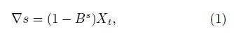
2 PRINCIPLE AND METHODS 2.1 Time Series (ARIMA Model) Method 2.1.1 Calculation of reference background valuesThe time series method (ARIMA model) applies the autoregressive integrated moving average model to analyze time series values,and find out the rule of them. Variations of total electric content (TEC) in the ionosphere are related with geographical location,seasons,local time,and activities of the sun and earth. So TEC values contain annual,seasonal,and daily periodical changes and random variations. In terms of this method,both certain and uncertain components of TEC values can be taken into account,thus the yielded reference background values can be more accurate.
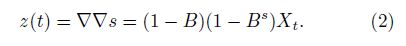
Figure1 shows modeling and calculation of TEC background values. First,we use the differential method to stabilize TEC sequence. Then we construct a seasonal model on stabilized sequence. At last,we find the optimal model based on AIC and SBC criteria and predict TEC reference background values. The specific procedures are as follows: First,differential calculation using period step s is conducted on TEC sequence,in which the period step is determined according to observations to sequence diagram and its autocorrelation function. The seasonal difference is

|
Fig.1 Flow Chart of modeling and predicting background values using the ARIMA model |
Then,we use ARIMA model to fit this sTable sequence[15]. In general,after a seasonal difference and a normal difference,the original sequence should be transformed into a stable time sequence z(t). If not,we continue such difference till it is stable. Finally,we check significance of the models,and evaluate all models checked using AIC or SBC criterion[16, 17],and find out the optimal model. With this model,we simulate TEC sample sequence of the ionosphere and obtain its reference background values.
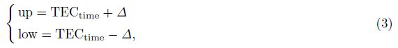
2.1.2 Calculation of limit values of background valuesWhen we calculate the upper and lower values of TEC background,we also use a more reasonable strategy in addition to the time series method (ARIMA model). First,we choose TEC data of the ionosphere close to an earthquake in location and time,which is not affected by sun flare and geomagnetic anomalies. Such TEC data should be at GIM grid points of or near the earthquake epicenter,and their time covers the 28 days from the 15th to 60th before the earthquake. And as much early to earthquake occurrence,the data are not influenced by the earthquake either. Then,choosing 20 days of the section as sample data,we use the time series method (ARIMA model) to predict the reference background values for 8 days after the sample days. Finally,we calculate the differences between these reference background values of 8 days and real observations,and the residuals which percentage of statistics predicted value of residuals is over 95.5% as the upper and lower values for the background. They are expressed as
The flow chart of ionospheric anomaly detection is shown in Fig.2. In brief,first,the upper and lower TEC values are determined. Then,the background values of TEC are predicted by the time series method. At last,anomalies are determined by differences between limited model values and observations. As a long time series will make prediction accuracy low,we adopt step-wise prediction,i.e. each time we calculate reference background for 7 days at most,then move forward the sample sequence (remove the data of foremost 7 days,and add just predicted data of 7 days to form a new sample sequence),and continue to make prediction. The newly added data may contain anomalies related to earthquakes. If so,such disturbed data must be removed from the sequence,and replaced by normal data through interpolation. Hence,the sample lengths can keep consistent.

|
Fig.2 Flow Chart of anomaly detection using the ARIMA model |
The conventional methods include the median,average,Inter Quartile Range,and sliding window. In the median method,the TEC data of the ionosphere in the earthquake month,are used and rearranged according to their magnitudes. Taking their median as the reference background value,and calculating standard deviation on it,we take 1.5 times the result as limit range for reference background. The average method takes the mean values of corresponding time in that month as the background value. Both the methods are of static detection,which does not remove disturbed values from sample data. Consequently,there are big discrepancy between the calculated background value and accurate values,making the detection very inaccurate[13]. So we do not compare them with our new method.
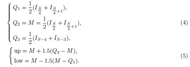
The Inter Quartile Range method was suggested by Liu et al.[11]. It chooses TEC data of S days (S can be divided with 4 exactly),arranges them in the order from small to large,and divided these data into four groups,of which the boundary point is denoted by Q1,Q2,and Q3. If the ordered data of S days are I1< I2· · · < Is,Q1,Q2,and Q3can be expressed by Eq.(4),and their upper and lower limits are as Eq.(5).
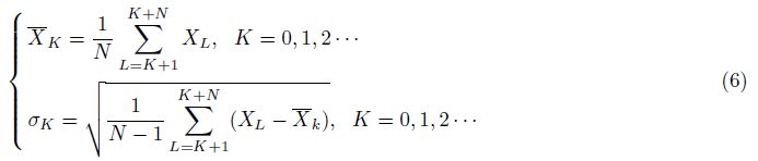
The sliding window is also relatively reasonable. It takes a proper window length for sliding,and calculates average and mean square errors. Taking the average as the basic value,it takes two times of the mean square errors as background range. The specific procedures are as follows. Let XL be TEC sequence of a station,take a sliding window length N. The window mean and upper and lower limits are calculated by
This sliding window and Inter Quartile Range method can predict background values more accurate relative to the median and average approaches aforementioned. Thus it can further calculate upper and lower limits of the background better. Particularly,the sliding window method can remove anomalous data in time. But because the accuracy of its predicted background values is limited,the final detection results are suspectable.
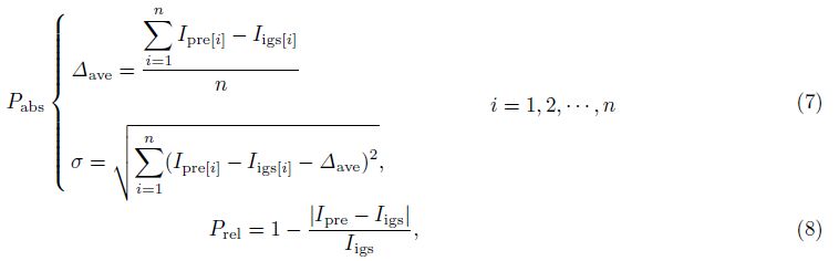
3 COMPARISON OF ACCURACY BETWEEN METHODSHere we compare the prediction accuracy of TEC background values by the time series method (ARIMA model) and conventional approaches. To the data of 22 November 2011 to 19 December 2011 (0°N,95°E) provided by IGS,we analyze their TEC sequence. Using the sliding window,Inter Quartile Range method,and the time series method (ARIMA model),we predict the background values of 12-19 December,respectively,and compare their accuracy. Here we adopt relative accuracy Prel and absolute accuracy Pabs{Iave,δ},which are defined as
As illustrated in Fig.3,the relative accuracy of prediction by the time series method (ARIMA model) is the best,next are the sliding window and Inter Quartile Range methods. Although they have similar accuracy at initial stage of prediction,with time increasing the time series method is conspicuously superior to the other methods. It is noted that some regular low-accuracy epochs are present in Fig.3 which are associated with extreme values in the TEC sequence predicted,nevertheless the comparison above still holds true.

|
Fig.3 Comparison of Relative prediction accuracy by time sequence method and traditional methods |
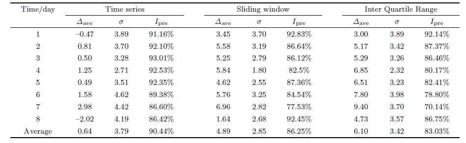
Table1 shows statistics of absolute and relative accuracy each day by the three detection methods. The comparison of its relative accuracy is consistent with Fig.3. In absolute accuracy,the average discrepancy of predicted background values by the time series method (ARIMA model) is pronouncedly better than the other methods,Though the standard deviation of the time series method is worse than the traditional methods,they do not differ much. And the background values predicted by the sliding window and Inter Quartile Range methods have large systematic discrepancies which would affect the ionosphere anomaly detection seriously. It means their detection results would be incorrect even if the limit error range is reasonably determined.
| Table 1 Statistics of absolute accuracy and relative accuracy of prediction results by the three methods |
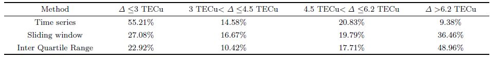
From Table2,the prediction residuals less than 6.2 TECu account for 90.62% for the time series method (ARIMA model),63.54% for sliding method,and 51.04% for Inter Quartile Range method,respectively. In terms of 3 TECu as criterion,the percentages of the first method are two times that of the other two approaches. It proves again that the time series method presented in this work is appreciably better than conventional methods.
| Table 2 Statistics of percentages in prediction residuals of the three methods |
In sum,several comparisons demonstrate that the time series method (ARIMA model) has much better accuracy in predicting background values of TEC with respect to conventional methods. So it can predict reasonable reference background values for normal TEC sequence as well as its error range.
4 CASE STUDY: SUMATRA M7.2 EARTHQUAKE 4.1 Data and Processing ProceduresOn 10 January 2012,a M7.2 earthquake occurred at the Sumatra island (epicenter 2.4°N,93.2°E,focal depth 19 km). Here we analyze disturbance in the ionosphere 13 days before and 1 day after this event. The TEC data used GIM grid product offered by IGS.
The data are processed by the procedures described in section 2.1 of this paper. First,we take the ionosphere TEC data from 9 December to 28 December 2011,20 days,as the sample sequence to predict reference background values of TEC from 29 December 2011 to 4 January 2012 (i.e. 13 to 7 days before the earthquake). Then,based on limit values determined by the method described in Section 2.1.2,we calculate the limit values for anomaly detection. As error statistics on reference prediction values from 12 December to 19 December 2011 for the time series method has been conducted (see Table2),and these data are close to the epicenter and occurrence time,not influenced by activities of the sun,geomagnetism and earthquakes,so the prediction residuals (±8.2 TECu) that account for 95.5% or more can be used as the error range for predicted background values for this event. At last,upon the principle in Section 2.1,we detect TEC anomalies by two steps. First,we analyze ionosphere anomalies from 7 days to 13 days before the Sumatra event. Then,we detect the anomalies in remaining 7 days in such a way that we slide the 20-day sample data forward for 7 days,i.e. removing foremost 7-day data,and add the data from 13 days to 7 days before the event into the sample sequence. Next,we delete anomalies from the new sequence,and replace them by normal values yielded with the neighboring interpolation.
Now we prove that there is no necessary relationship between the ionosphere anomalies and other variations such as activities of the sun,geomagnetic field and weather 13 days before the Sumatra earthquake on 10 January 2012. Fig.4 shows the Kp index for geomagnetic activity and Dst index for ring current intensity during the period aforementioned. Usually,Kp index less than 3 means the quiet ionosphere,Dst smaller than -50 nT indicates possible medium-level magnetic storms,and Dst less than -100 nT implies likely great magnetic storms. From Fig.4,Kp and Dst indexes are at low levels. Thus it can be concluded that there were no influence of the sun and geomagnetic field and other factors on the ionosphere 13 days before and 1 day after the Sumatra earthquake. If ionosphere anomalies during this period are detected,they were very likely produced by the earthquake.

|
Fig.4 Kp and Dst indexes during the detection period (29 December 2011 to 11 January 2012) before the Sumatra earthquake |
We used 4 GIM grid points around the epicenter to examine ionosphere TEC anomalies 13 days before and 1 day after the Sumatra earthquake (Fig.5).

|
Fig.5 Results of TEC anomaly detection using ARIMA model (left) and IQR method (right) In each diagram, upper is anomaly detection sequence, blue dotted line is anomaly limit values, red dotted line is real observed values; lower is differences between observed and normal values, red column is positive anomaly, i.e. higher than upper limit, blue column is negative anomaly, i.e. lower than limit. |
As shown in Fig.5,the detection results by the time series method and sliding window method differ much. The anomaly days from the latter are more than the former. And from the latter approach,anomalies occurred continuously once it come about,and there is no obvious regularity in its positive and negative values. This is associated with the fault in the sliding window method itself. Because in this method,the accuracy of reference background values for prediction is low,and their error limits are unreasonable. It can also explain the limitation of conventional methods in studying pre-seismic ionosphere anomalies.
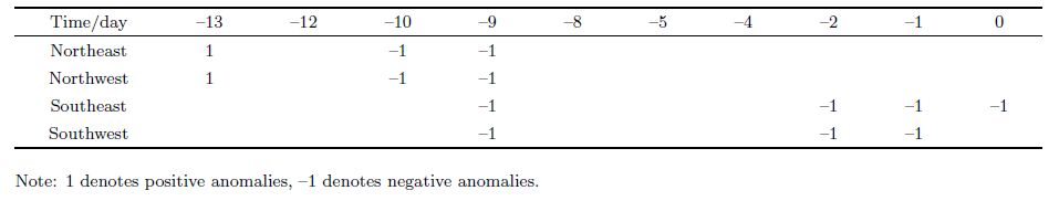
Because of problematic accuracy and reliability in the detection results from the sliding window methods,here we only make detailed analysis to the ionosphere anomalies from the time series technology. On the 13th day before the earthquake,pronounced positive anomalies occurred at D1 point (northeast),and negative anomalies appeared there at the 9th to 10th day before the event. The anomalies at D2 (northwest) are roughly consistent with D1. At D3 (southeast),negative anomalies were seen on the 9th,1st to 2nd day before the event and the day of the earthquake. D4 (southwest) is largely same as D3. Their statistics is listed in Table3,in which 1 denotes positive anomalies,and -1 denotes negative anomalies. It is clear that at the 13th day before the event,considerable positive anomalies only occurred north of the epicenter,while no such phenomenon appeared in south. In contrast,negative anomalies are seen in four directions around the epicenter,which occurred at the 9th,10th,1st and 2nd day before the event and the day of the earthquake. In sum,anomalies were observed north to the epicenter at a time relatively earlier to the earthquake occurrence,while negative anomalies were notable in south,and close to earthquake occurrence time.
| Table 3 Anomaly statistics in all directions before the event and when the earthquake happened |
To further reveal regularity of seismic anomalies,we make statistics of occurrence frequencies of all anomalies in four time sections of one day,which are GMT 0:00-6:00 (LT 7:00-13:00),GMT 6:00-12:00 (LT 13:00-19:00),GMT 12:00-18:00 (LT 19:00 to 1:00 next day),GMT 18:00-24:00 (LT next day 1:00 to next day 7:00),here GMT is international time,LT is local time (Fig.6). The results show that the occurrence frequencies of anomalies gradually increase in the first,second,and third section,while that is lowest in the fourth section. Relative to earthquake occurrence time (GMT 18:36),time section 3 is closest before the event,and time section 4 is the closest after the event. Prior to the earthquake,the closer to the earthquake occurrence time,the more frequent anomalies are. While after the event,the least anomaly frequency occurs at the fourth time section that is closest to the earthquake occurrence time. The third time section with highest frequency of anomalies was local time 19:00 to 1:00 next day,during which there was little influence of solar activity. Therefore,it can be inferred that the regularity above is likely related with the Sumatra earthquake,though it needs further research upon more data. If such regularity exists indeed,it would be of importance for predicting occurrence time (with accuracy to hours) of earthquakes.

|
Fig.6 Percentage statistics of anomalies in four time sections of one day |
This paper proposes the time series method (ARIMA model) for detection of pre-seismic ionosphere anomalies. We present its principle and flow in detail,and compare with conventional methods in prediction accuracy of background values and other features. The results show that the accuracy of predicting background values by this new method is remarkably better than that of the Inter Quartile Range and sliding window methods,the latter have large discrepancy which can influence subsequent detection seriously. Besides,this work suggests a more reasonable strategy to determine limit values. In terms of the precise background values and reasonable upper and lower limit values,we can obtain more reliable results of anomaly detection and explanation. Finally,we use the time series method (ARIMA model) to analyze ionosphere TEC disturbance associated with the Sumatra M7.2 earthquake on 10 January 2012.
(1) On 13th day before and 1st day after the event,there existed indeed ionosphere anomalies observable,which were not influence by other factors such as solar and geomagnetic activity. It means that anomalous disturbance in the ionosphere to some extent can be generated before a major earthquakes. Hence,observations and analysis to such a phenomenon may be a tool to realize short-term and impending earthquake prediction.
(2) From the case study of the Sumatra event,ionosphere anomalies would occur on the 13th,8th to 9th,1st to 2nd day and several hours before the earthquake. The normal anomalies mainly occurred north of the epicenter,and earlier to the earthquake occurrence time,which are not evident in south of the epicenter. The negative anomalies appeared in all four directions several days and 8~4 h before the event,and closer to the earthquake time.
(3) The statistics on time sections of one day indicates that more frequent anomalies occur at the time closer to the earthquake time before the event,while after the event,less frequent anomalies closer to the earthquake time. This regularity needs further studies. If it exists indeed,this would provide important reference for predicting earthquake occurrence time (with accuracy to hours).
By means of more accurate TEC anomaly detection,this work attests to the existence of pre-seismic ionosphere disturbance,and the feasibility of earthquake prediction using such a phenomenon. It requires,however,further studies because of complicated mechanisms for earthquakes as well as for pre-seismic ionosphere perturbation.
6 ACKNOWLEDGMENTSThe ionosphere TEC data,Kp index and Dst index used in this paper were provided by IGS,NGDS of US,and Geomagnetic Center of Kyoto,Japan. This work was supported by the National Natural Science Foundation of China (41074024) and Science Foundation for Innovative Research Groups (41021061).
| [1] Astafyeva E,Heki K.Vertical TEC over seismically active region during low solar activity.J.Atmos.Sol.-Terr.Phys.,2011,73(13):1643-1652. |
| [2] Chavez O,Prez-Enrquez R,Cruz-Abeyro J A,et al.Detection of electromagnetic anomalies of three earthquakes in Mexico with an improved statistical method.Nat.Hazards Earth Syst.Sci.,2011,11:2021-2027,doi:10.5194/nhess-11-2021-2011. |
| [3] Hasbi A M,Mohd Ali M A,Misran N.Ionospheric variations before some large earthquakes over Sumatra.Nat.Hazards Earth Syst.Sci.,2011,11:597-611,doi:10.5194/nhess-11-597-2011. |
| [4] Oyama K I,Kakinami Y,Liu J Y,et al.Reduction of electron temperature in low latitude ionosphere at 600 km before and after large earthquakes.1J.Geophys.Res.,2008,113:A11317,doi:10.029/2008ja013367. |
| [5] Barnes R A,Leonard R S.Observations of ionospheric disturbances following the Alaska earthquake.J.Geophys.Res.,1965,70:1250-1253. |
| [6] Pulinets S A,Contreras A L,Ciraolo L,et al.Total electron content variations in the ionosphere before the Colima,Mexico,earthquake of 21 January 2003.Geofisica Internacional,2005,44(4):369-377. |
| [7] Datchenko E A,Ulomov V I,Chernyshova C P.Electron density anomalies as the possible precursor of Tashkent earthquake.Dokl.Uzbek.Acad.Sci.,1972,12:30-34. |
| [8] Meng Y,Wang Z M,E D C.Ionopsheric TEC anomalies of pre-earthquake based on GPS data.Geomatics and Information Science of Wuhan University(in Chinese),2008,33(1):81-84. |
| [9] Lin J,Wu Y,Zhu F Y,et al.Wenchuan earthquake ionosphere TEC anomaly detected by GPS.Chinese J.Geophys.(in Chinese),2009,52(1):297-300. |
| [10] Cai J T,Chen X B,Zhao G Z,et al.Earthquake precursor:the anomalies in anomalies in the ionospheric F2 region.Progress in Geophysics(in Chinese),2007,22(3):720-728. |
| [11] Liu J Y,Chen Y I,Pulinets S A,et al.Seismo-ionospheric signatures prior to M≥6.0 Taiwan earthquakes.Geophys.Res.Lett.,2000,27(19):3113-3116. |
| [12] Pulinets S A,Legen'ka A D,Gaivoronskaya T V.Main phenomenological features of ionospheric precursors of strong earthquakes.Atmos.Sol.Terr.Phys.,2003,65():1337-1347. |
| [13] Zhu F Y,Wu Y,Lin J,et al.Study on ionospheric TEC anomaly prior to Wenchuan Ms8.0 earthquake.Journal of Geodesy and Geodynamics(in Chinese),2008,28(6):16-21. |
| [14] Yao Y B,Chen P,Zhang S,et al.Analysis of pre-earthquake ionospheric anomalies before the global M=7.0+ earthquakes in 2010.Nat.Hazards Earth Syst.Sci.,2012,12:575-585. |
| [15] James D.Hamilton.Time series Analysis.Princeton University Press,1994. |
| [16] Wang Y.Application of Time Series Analysis(The second edition).Beijing:People's University of China Press,2008. |
| [17] He S Y.Application of Time Series Analysis.Beijing:Beijing University Press,2007. |