1 INTRODUCTION

The ionosphere is a region where the low-orbit satellites are mainly orbiting the Earth and is also the main area where space weather affects human’s life. Ionospheric disturbances caused by solar storms can affect the accuracy of the Global Positioning System (GPS), the quality of radio communication and the safety of the power transmission. Most of missiles, low-orbit satellites and space stations run in the ionosphere, the state of which will directly affect the lifetime of the spacecrafts and the fulfillment of their functions, as well as the health and safety of the astronauts^[1]. Since ionospheric disturbances with quick changes and large dynamic range take place from time to time, it is of great significance to effectively monitor the status of the ionosphere, especially its electron density profile, EDP and total electron content, TEC. The traditional detecting techniques are conditioned by sites distribution, acquisition time and work frequency, so that they cannot meet the high resolution need of global detection. For example, ionosondes are confined to the lower ionosphere, while incoherent scatter radar could detect the ionosphere below 800 km and provide several parameters, but its maintenance costs too much. From 1970s, NASA began to develop a remote sensing technique which applies far ultraviolet spectrographs to measure aurora and airglow radiation in the ionosphere, and it aroused much attention of researchers for its high resolutions in space and time. In the past decades, many researchers did lots of studies on how to retrieve ionospheric parameters from measurements of far ultraviolet spectrographs^{[2, 3, 4, 5, 6, 7]}. As for the retrieval problem of EDP from far ultraviolet airglow, most of these studies abroad were performed under the assumption that EDP follows Chapman function, which resulted in a big deviation in both peak electron density and peak height. While in China, researches on this question have just begun. Finding an effective method to retrieve EDP from far ultraviolet spectroscopic measurements can not only enrich the database of ionospheric observations, but also serve some technical advice for quickly transforming homogenous data in our country to data products. Based on the OI 135.6 nm measurements obtained by Global Ultraviolet Imager aboard on TIMED spacecraft, this work applied a combined method of regularization and Newton-iteration to calculate the free-form ionospheric EDP. Afterwards, it combines the peak electron density and peak height of the free-form ionospheric EDP with the Chapman expression and the Chapman-fitted EDP is yielded.

2 DATA AND OBSERVATIONAL MODEL 2.1 Data Description

GUVI^[8] has provided spectrometric data of the ionosphere since its launch to near-polar sun-synchronous orbit aboard on TIMED spacecraft in December, 2001. It circled the Earth with a period of 97.8 min, an altitude of 625 km and an inclination angle of 74.1°. Its limb observations of OI 135.6 nm nightglow were used to retrieve EDP, whose volume emission rate can be expressed as

where ε_mn is the contribution of neutralization reactions in OI 135.6 nm nightglow, and R₁ = 7.3×10^-13, R₂ = 10^-7, R₃ = 1.3 × 10^-15, R₄ = 1.4 × 10^-10 are the rates of the corresponding reactions, all in unit of cm³/s.

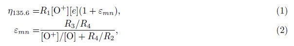
As shown in Fig.1, the atmospheric model NRL MSISE-00 and International Reference Ionospheric Model IRI-2001 were used to calculate the contribution of neutralization reactions, ε_mn, at (30°N, 0°E) for March 21, 1992. Radiative recombination reactions account for 75% of the measured OI 135.6 nm intensities, the remaining 25% are mainly from neutralization reactions^{[9, 10, 11]}. From Fig.1 we can see that neutralization reactions become a factor only below 250 km, therefore, assuming that the measured OI 135.6 nm intensities only originate from radiative recombination reactions, the influence of neutralization reactions is neglected in the subsequent calculations. Additionally, assuming that O⁺ is the dominant ion in F region (its content is above 99%) and that the ionosphere is electrically neutral, then O⁺ density equals the electron density, that is

Thus, the volume emission rate η can be rewritten as where [e] represents the electron density.

2.2 Observational Model

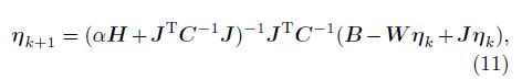
The scanning and imaging system of GUVI scans the limb area with a range of 67.2° to 80° from nadir viewing at a step of 0.4° along the cross-track when TIMED runs along its track, obtaining 32×14 pixels. The imaging geometry of GUVI is shown in Fig.2. Each pixel is the sum of the radiation along the line of sight from the tangent point to the observer. To remove the influence of random noise, 14 pixels along the track are averaged. Therefore, 32 pixels of one scan are related to 32 tangent altitudes. If assuming the ionosphere is spherically symmetric, the ionosphere from 90 km to 530 km can be divided into 23 layers and the observational model of discrete form can be established as follows

For one scan, the observing vector B is a column vector of 32 elements; the weighted matrix W is 32×23, each element in each row of W is the ratio of the radiation of the corresponding layer to the measured intensities; the volume emission rate η is a column vector of 23 elements and N is the additive noise.

2.2.1 Analysis of noise

The additive noise N is dominated by photon shot noise, thus only the influence of photon shot noise is considered in this article. Photon shot noise is relevant to the incoming photon counts. Statistically, the noise behaves according to a Poisson distribution, photon shot noise σ_shot can be represented by the square root of signal electron counts S_e (the number of electrons):

The sensitivity of GUVI for 135.6 nm is 0.5 counts/s/Rayleigh/pixel, the integration time is 0.064 s, as the discrete model uses the averaging of 14 pixels, then the additive noise could be expressed in Eq.(7) and B takes the values of observation vector in Eq.(5).

2.2.2 Weighted matrix

The observational model is established under the assumption that the ionosphere is spherically symmetric. Each element of a row in the weighted matrix is only related to the distance between each corresponding layer and the instrument^[12]. Thereupon, the weighted matrices of all the locations are identical in the observational model. The condition number of matrix W^TW is 3469, which will directly affect the accuracy of retrieval results. It is generally believed when the condition number is less than 100 it is well-conditioned, when that is between 100 and 1000 it is moderate ill-conditioned and when that exceeds 1000 it is seriously ill-conditioned^[13]. It is obvious that the retrieval problem of EDP involved in the research is seriously ill-conditioned.

As a result, based on the limb viewing model established above, the retrieval problem of EDP could be transformed into a least-squares estimation as follows

where b is a vector of the differences between the measurements and the noise. However, because of the illconditioning of the weighted matrix in the model, the estimated solution by the least-squares estimation method deviates from its true value. In this study, the regularization method is applied to solve that problem by means of adding a side constraint.

3 RETRIEVAL METHOD

Tikhonov put up with a regularization method to solve the aforementioned ill-posed problem. The regularization method overcomes the ill-posedness to ensure the uniqueness and stability of the solution by means of incorporating the minimum of the weighted sum of squares of some parameters or corrected parameters, that is, using the solution of an adjacent well-posed problem to approach the optimal solution of the original problem. Hence, to ensure the Eq.(8) has a unique and stable solution, a criterion function is built

where the parameter η that minimizes the Eq.(9) is the regularization solution of the established observing model. Here, the side constraint Ω(η) is called a stable function and α is regularization parameter, smoothing factor or ridge parameter. In the calculation, the side constraint Ω(η) takes different forms. In this study, Ω(η) = η^THη and the regularization matrix H = D₂^T D₂. D₂ usually takes the first-order or second-order differential of identical matrix, Laplace operator, and here the second-order differential of Laplace operator is applied At present, the L-curve method and Generalized Cross-Validation method are commonly used to determine the regularization parameter^[14] and the latter was adopted in this paper. Since ..Wη - b..₂ and ..D₂η..₂ are both functions of regularization parameter α, given a series of different α, with ..Wη - b..₂ and ..D₂η..₂ being horizontal and vertical coordinates, L-curve shown in Fig.3 is obtained by curve fitting.

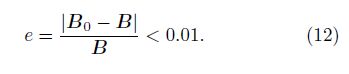
Newton-iteration procedure is adopted to find the optimal solution of the unknown η, for it has the property of rapid convergence. The iterative formula^[15] is

where J is the Jacobian matrix of Wη at η_k, and C is the covariance matrix of the noise. The Eq.(11) is iterated when the following condition is met, and B₀ is the estimated values of the radiance

4 RESULTS AND ANALYSIS 4.1 Comparison with Ground-Based Measurements

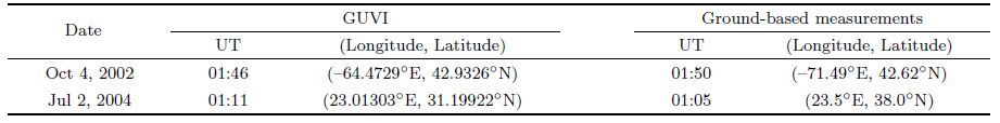
Free form ionospheric EDPs of Oct 4, 2002 and Jul 2, 2004 are retrieved from the selected GUVI limb viewing OI 135.6 nm nightglow radiance data that have near-synchronous ground-based observations by means of regularization combined with the Newton-iteration method. The detailed parameters of Oct 4, 2002 and Jul 2, 2004 are listed in Table1. The retrieved EDPs, together with EDPs derived from ground-based observations and Full Analytic Ionospheric Model (FAIM)^[16] are plotted in Fig.4. The ground-based EDPs of Oct 4, 2002 are from Millstone Hill Incoherent Scatter Radar, ISR, while Athens ionosonde only provides the peak electron density and peak height and the EDPs on Jul 2, 2004 are fitted with Chapman function.

As shown in Figs. 4a and 4c, compared to FAIM, the results derived in this paper are closer to those from ground-based measurements above 200 km; but in the region below 200 km, they have a greater difference. This phenomenon is likely due to: neutralization reactions are not involved below 200 km and GUVI measurements differ from those ground-based in space and time, about 7° difference in longitude. There is a greater difference in the retrieved EDPs below 200 km, but the peak electron density and peak height agree well with the referenced EDPs.

Usually, Chapman function is used to characterize the EDP in the ionosphere^[17]

where z is altitude; N_m and h_m represent peak electron density and peak height respectively and the scale height H here takes 54 km. Chapman-fitted EDPs shown in Figs. 4b and 4d are obtained by substituting peak electron density and peak height calculated before into the Eq.(13). From Figs. 4b and 4d we can see that the derived EDPs by substituting peak electron density and peak height calculated by the proposed regularization algorithm into Chapman function agree very well with the ground-based measurements.

In summary, the free-form EDPs obtained from measurements of OI 135.6 nm nightglow through the regularization and Newton-iteration method take an obvious advantage over FAIM, while they have certain differences with the ground-based results below 200 km. Nevertheless, the peak electron density and peak height agree very well with those from ground-based instrument. Therefore, the algorithm proposed in this paper can compensate for the weaknesses of the traditional method. For example, sites of incoherent scatter radars and ionosondes are so scarce that they cannot provide the global structure and characteristics of ionospheric EDPs with high spatial resolution.

4.2 N_mF₂ Variation with Magnetic Storms

OI 135.6 nm measurements at 5°N between Sep 29 and Oct 3, 2002 are processed with the algorithm proposed in this paper, after which the variation of N_mF₂ with magnetic storms is researched. Internationally, according to Dst index, the magnetic storms could be classified as: weak storms (-50 < Dst ≤ -30), moderate storms (-100 < Dst ≤ -50), intense storms (-200 < Dst ≤ -100) and super storms (Dst ≤ -200). Dst indices from Sep 29 to Oct 3, 2002 are plotted in Fig.5. Sep 29 was magnetic quiet, weak storms occurred on Oct 1, and Oct 2 and 3 were in recovery phase, with Dst returning to its normal value.

The retrieved EDPs for Sep 29-Oct 3, 2002 are plotted in Fig.6. The exact longitude and acquisition time are labeled under the horizontal axis, and when there is a track lost, neighbor interpolation method is used to obtain the needed data and the corresponding longitude and acquisition time are not labeled. Here, referred to Fig.6a, a preliminary analysis of magnetic storms effect on ionospheric electron density has been performed.

Dst index decreased significantly since 04:00 UT in the early morning on Sep 30, and fluctuated around -20 nT until 10:00 UT. As shown in Fig.6b, equatorial anomalies occurred at longitudes from 208° to 257°, and the peak electron density was obviously higher than that of yesterday. A weak storm happened from 13:00 UT to 20:00 UT and slight increase of the electron density was found.

As shown in Fig.6c, when Dst index was fluctuated in a range of -20 nT to -40 nT from 03:00 UT to 10:00 UT on Oct 1, the ionospheric equatorial anomaly expanded largely near the longitudes from 201° to 299° of the Western Hemisphere. Afterwards, Dst index decreased rapidly, reached the minimum around 17:00 UT and remained -160 nT up and down until midnight, with the electron density of ionospheric F layer widely increased and uplifted.

Dst index in Fig.6d from midnight to 16:00 UT on Oct 2 were lower than Oct 1, the ionospheric equatorial anomaly near the longitudes from 242° to 291° of the Western Hemisphere extended to a larger scope, but the electron density at longitudes from 193° to 242° decreased. Dst index returned to its normal values after 16:00 UT and peak height or peak electron density decreased in a wide range. Dst index continued to pick up on Oct 3, and as shown in Fig.6e the equatorial anomaly was weakened.

By analyzing the variations of EDPs at 5°N from Sep 29 to Oct 3, 2002 in magnetic storms, we find that ionospheric equatorial anomalies will appear in the vicinity of the peak height with the occurrence and changes in the strength of the magnetic storm, whose degree and extent will vary at different longitudes.

5 CONCLUSIONS

Based on OI 135.6 nm nightglow measurements of GUVI, a limb-viewing model is established and the free-form ionospheric electron density is calculated by means of regularization combined with Newton-iteration method. After that, the peak electron density and peak height of free-form EDPs are combined with Chapman function to obtain Chapman-fitted EDPs and the fitted EDPs are compared with the corresponding data from ground-based instruments and FAIM. The results demonstrate that the retrieved EDPs agree very well with those from ground-based instruments above 200 km, but have some deviation from those below 200 km. The reason for this phenomenon needs to be further studied.

EDPs at the latitude of 5°N from Sep 29 to Oct 3, 2002 are derived with the algorithm presented in this paper and based on the retrieved EDPs, a preliminary analysis of the effects of magnetic storms on ionospheric electron density was performed. It is found that with the occurrence and changes in the strength of the magnetic storm, ionospheric equatorial anomalies will appear in the vicinity of the peak height, whose degree and extent will vary with different longitudes.

ACKNOWLEDGMENTS

This study was supported by the National Natural Science Foundation of China (40804048) and the National Key Basic Research Program 973 project (2013CB329202, 2009CB724005).