 2018, Vol.38


大量的研究表明,在全球主要的造山带(如喜马拉雅山脉、安第斯山脉、落基山脉等),不仅新生代构造活动强烈,降水、冰川等外力作用也十分显著[1~5]。因此,活动造山带的地形地貌特征是构造运动与气候变化相互作用的产物。河流作为造山带区域重要的地貌单元,对构造-气候的耦合作用最为敏感,无论是流域几何形态还是河道高程剖面,都受到构造、气候、岩性等的影响;同时,这些因素及其变化特征也为河流系统所记录。如何定量化研究河流地貌,从中获取区域构造活动特征,是构造地貌研究的热点[6~11]。
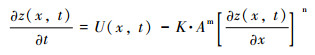
基岩河道水力侵蚀模型(stream-power river incision model)[6~7]为解决这一问题提供了一个良好的途径,促使构造地貌学的研究迈入一个崭新的阶段。该模型以基岩隆升速率与河水动力侵蚀速率之差表示河道高程的变化,从而将构造活动、河流侵蚀与地形变化三者相结合,使得可以通过河道高程剖面形态研究区域构造活动。该模型的数学表达如公式(1)所示[6~7]:
|
(1) |
其中,z为河道高程,t表示时间,x是从出水口到河道上某一点的溯源距离,U是基岩隆升速率,K是侵蚀系数(一般与岩性、气候和侵蚀方式有关),A是汇水面积,m和n分别为汇水面积和坡度的指数因子。
显然,这是一个复杂的非线性偏微分方程。直接求解这个方程比较困难,因此绝大多数的研究主要基于稳态(steady state),也称为均衡状态的河道高程剖面,即河道高程不随时间变化,这样公式(1)就转化为稳态形式[7]。通过稳态方程计算河道陡峭系数,可以用于表征区域隆升速率的空间分布特征[9~24]。
然而,就实际情况而言,大多数流域的基岩抬升速率与河流下切速率未达到平衡,此时河道处于非稳态(unsteady state,也称为非均衡状态或瞬态transient state)[25~31]。尤其对于流经断裂带的河流,断层滑动造成上升盘抬升,河道高程剖面上相应地会生成裂点[31~33]。随着时间推移,裂点溯源迁移,河道高程也会相应地产生一系列变化[32]。这些裂点有着怎样的运动规律?裂点迁移对河道有怎样的影响?如何从这些存在裂点的非稳态河道中提取构造活动信息?要回答这些问题,就必须对瞬态方程开展研究。鉴于这方面的研究需要以稳态方程为基础,所以本文将首先简要介绍稳态方程的相关研究方法,然后以此为基础,详细阐述现今国内外对于非均衡河道高程剖面的研究进展。
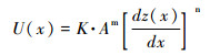
1 稳态方程当流域的基岩抬升速率与河流侵蚀速率相平衡,河道高程不再发生变化,河道处于稳态[15~17]。此时,方程(1)可以转化为稳态方程[17]:
|
(2) |
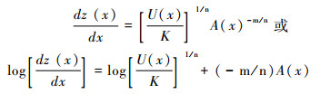
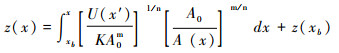
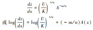
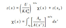
显然,当河道处于稳态时,隆升速率虽然不随时间变化,但可以随空间变化[17, 33]。从数学角度,公式(2)是一个关于河道高程z的一阶常微分方程,对于这个方程,有两种处理方法,分别称为坡度-面积法[16](公式3)和积分法[17](公式4):
|
(3) |
|
(4) |
其中,z(xb)为河道xb点处的高程,是方程(2)的边界条件;A0是参考汇水面积(可取任意值)。ks=[U(x)/K]1/n为河流陡峭系数(steepness index),θ=m/n为河流凹度(concavity)。显然,陡峭系数与基岩隆升速率成正比,因此可用于表示隆升速率的空间分布特征[9~24, 34];而河道凹度主要受到岩性的影响,与隆升速率的关系并不显著[10, 16~17, 34]。
如果流域的基岩隆升速率空间均匀,则公式(3)和(4)可简化为[16~17]:
|
(5) |
|
(6) |
公式(3)或(5)所示的坡度-面积法,是通过线性回归坡度-汇水面积的对数值来计算凹度和陡峭系数。而积分法(公式(4)或(6))直接求解稳态的水力侵蚀方程,得到河道的函数表达式。其中,对汇水面积的积分值称为χ值,所以这种方法又称为χ-z plot(也写作Chi plot)[17]。线性回归χ值与河道高程,其斜率就是河道陡峭系数。关于这两种方法各自的优缺点,笔者曾作过详细分析,并提出相应的改进措施[35],但这并不是本文重点,故不赘述。
公式(5)和(6)表明,当河道处于稳态,并且流域基岩隆升速率空间均匀时,河道的坡度-面积对数图和χ-z plot都具有良好的线性关系。但需要注意的是,这二者之间并不存在严格的因果关系[35]。例如,Kirby和Whipple[34]在研究位于喜马拉雅前缘地带Siwalik背斜时发现,尽管流域基岩隆升速率空间非均匀,河流的坡度-面积对数图也存在较好的线性关系。Wang等[35]在研究美国加州北部MTJ(Mendocino Triple Junction)区域的河流时,发现河道岩性的差异,会造成某些稳态河道的χ-z plot偏离线性关系。
2 裂点溯源迁移规律与地貌响应时间河道处于非均衡状态,最显著的标志是河道出现裂点[26, 33]。裂点,即河道高程剖面上坡度不连续点[26],可以通过坡度-面积对数分布图或者河道的χ-z plot识别[25~29, 33~37]。按照不同的分类标准,可以将裂点分为很多类型。不同类型的裂点,其运动规律是有差别的[38]。本章首先简介裂点类型,然后着重阐述构造成因裂点的溯源迁移规律,以此计算流域的地貌响应时间,最后介绍裂点迁移对河道的改造。
2.1 裂点类型Kirby和Whipple[38]按照裂点是否发生溯源迁移,将裂点划分为移动型与固定型两类;按照裂点对其下游河道的改造结果分为Vertical-step和Slope-break两类。Vertical-step型裂点,河道坡度仅在裂点附近局部区域陡增,而裂点上、下游河道陡峭系数相同(图 1a和1c);Slope-break型裂点则不同,其上、下游河道陡峭系数发生明显改变,河道坡度增加不仅仅局限在裂点附近(图 1b和1d)。

|
图 1 Vertical-step型和Slope-break型裂点在河道高程剖面和坡度-面积对数图上的区别(据文献[38]修改) Fig. 1 The difference between Vertical-step and Slope-break knickpoints on river profiles and log-transformed slope-area plots, modified from reference[38] |
当河道局部区域(其尺度相对于流域整体规模而言很小)的岩石抗侵蚀能力增强(说明河道侵蚀系数K减小),则该区域的河道坡度会大幅增加以保持恒定的侵蚀速率,这种情况下可能会形成固定的Vertical-step裂点;当河流流经岩性差异显著的区域,会造成河道侵蚀系数的显著改变,这样导致河道不同岩性河段的陡峭系数发生明显改变,这种条件下容易形成固定的Slope-break裂点。由此可见,固定型裂点大多与岩性差异有关[38]。但需要注意的是,并不是所有的固定型裂点都是岩性差异造成的。例如Regalla等[39]在研究日本Abukuma山区时发现,断层几何形态的改变,会造成区域隆升速率的空间变化,这种情况下可以形成稳定的裂点;我国的雅鲁藏布大峡谷,就是一个稳定的巨型裂点,其主要成因便是峡谷附近地壳的差异隆升[2, 40]。
当气候干旱造成河流局部侵蚀基准面(如小型湖泊)下降,河流会在基准面附近形成裂点,该裂点在溯源迁移的过程中一般仅仅造成裂点局部区域坡度增加而不会改变河道整体的陡峭系数,这种裂点称为移动的Vertical-step裂点;在活动造山带,断层滑动造成区域隆升,相应的,该区域的河流在流经断层的位置会产生裂点,裂点溯源迁移并改变其经过的河道的陡峭系数,这种裂点就是移动的Slope-break裂点。这种构造成因裂点的溯源迁移规律,在计算流域地貌响应时间,求解非稳态的水力侵蚀方程,从河道高程剖面中提取区域岩体隆升历史等方面有着重要作用[26, 32~33, 36, 41~44],是现今构造地貌研究的重要内容,也是本文介绍的重点。其余类型裂点大多与岩性、气候等相关,研究这些裂点的运动规律对于模拟区域隆升历史并无太多助益,因此本文不作深入讨论。
2.2 裂点溯源迁移速率Berlin和Anderson[26]假设河流侵蚀速率与河道坡度呈线性关系(即n=1),同时流域内岩体隆升速率空间均匀,推导得出了移动型Slope-break裂点溯源迁移速率的水平分量。这一结果被广泛用于线性瞬态方程的求解和模拟区域岩体隆升历史[32~33, 35, 44]。笔者[40]推导了复杂条件下(n≠1,并且区域岩体的隆升速率空间非均匀),裂点溯源迁移速率的水平和垂直分量。本文主要介绍笔者的模型和推导过程。
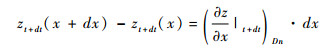
如图 2所示,河道裂点附近局部河段的示意图。在t时刻,河道各处的基岩抬升速率以Ut(x)表示,裂点处于A点位置;经过dt的时间间隔,基岩抬升速率变化为Ut+dt(x),裂点从A点溯源迁移到D点。尽管图 2表示的是流域基岩抬升速率随时间增加的情况,但当抬升速率随时间降低时,以下公式(7)~(20)也适用。

|
图 2 裂点溯源迁移模型 在t时刻,裂点处于A点,经过dt时间间隔溯源迁移至D点;实线表示t时刻河道高程剖面,浅灰色虚线表示t+dt时刻河道高程剖面(据文献[40]修改) Fig. 2 Knickpoint migration model, modified from reference[40]. A knickpoint locates at point A on time t and migrates to point D in a time step dt. The dark solid line indicates a river profile in time t. The light gray dashed line indicates a river profile in time t+dt |
由于区域构造隆升,河道的高程剖面也由原先的zt变化为zt+dt。那么裂点的高程变化可以表示为:

|
(7) |
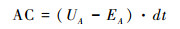
AC、BD分别表示A点和B点的河道基岩隆升速率与侵蚀速率差。BG是t时刻河道剖面上A、B两点的高程差。它们可以表示为:
|
(8) |
|
(9) |
|
(10) |
|
(11) |
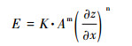
其中,U是基岩隆升速率(UA、UB分别是t时刻,裂点下游、上游河段的基岩隆升速率);E为侵蚀速率。下标Dn表示裂点下游河段,Up表示裂点上游河段。vH表示裂点溯源迁移速率的水平分量。同时,根据河水动力侵蚀模型,侵蚀速率可以表示为侵蚀系数K、汇水面积A和河道坡度的函数:
|
(12) |
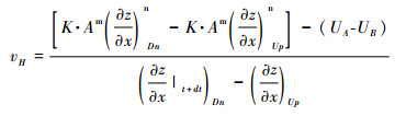
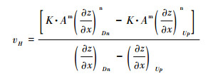
将公式(8)~(12)代入公式(7),可以得到裂点溯源迁移速率的水平分量vH:
|
(13) |
由公式(13)可知,当裂点下游、上游河段的基岩隆升速率差不小于侵蚀速率差时,裂点会保持稳定。这就是当区域岩体隆升速率空间非均匀时,裂点保持稳定的临界条件。Wang等[40]根据这个临界条件,研究雅鲁藏布大峡谷稳定的原因,从理论上支持了Wang等[2]提出的“大峡谷缘于其附近地壳差异隆升”的观点。
当流域内基岩隆升速率空间均匀(UA=UB)时,则裂点所经过的河道保持与新的隆升速率相平衡,河道坡度不再发生变化[33]。那么,vH可以简化为:
|
(14) |
分子分母同时乘以(K·Am)1/n,得:
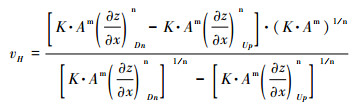
|
(15) |
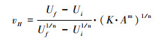
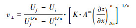
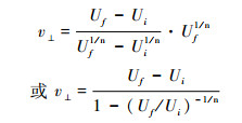
裂点在溯源迁移过程中,其所经过的河道将达到与新的隆升速率(以Uf表示)相平衡的状态,而裂点以上的河道仍保持与原先的隆升速率(以Ui表示)相平衡的状态。因此,公式(15)又可以表示为:
|
(16) |
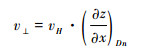
裂点溯源迁移速率的垂向分量(v⊥)与水平分量(vH)的比值是裂点坡度的正切值,即:
|
(17) |
将公式(17)代入公式(16),得:
|
(18) |
裂点下游河段侵蚀速率已经保持与基岩隆升速率相平衡。则,公式(18)也可如下:
|
(19) |
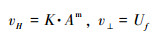
当河流侵蚀速率与河道坡度呈线性关系(n=1),裂点溯源迁移速率的水平和垂向分量分别可以简化为:
|
(20) |
显然,公式(20)的结果与前人[26, 33]的研究是一致的。对于线性情况(公式(20)),裂点的水平运动速率仅取决于侵蚀系数和汇水面积。这就是说不同时期形成的裂点将以相同的水平速率溯源迁移,不会发生早期裂点被“吞并”的现象,区域的隆升历史也可以被完整地保留在河道高程剖面上。这与Royden和Perron[32]的推论是一致的。
而由公式(16)和(19)可见,对于非线性条件,裂点溯源迁移速率受到裂点生成时和生成前的基岩隆升速率的影响。因而,不同时期生成的裂点,其溯源迁移速率存在显著差别,早期形成的裂点有可能被后期的裂点“吞并”。此时,会造成区域隆升历史的信息缺失[32]。
2.3 裂点迁移对河道高程剖面的影响与地貌响应时间Goren等[33]说明了裂点迁移对河道高程剖面的影响。假设初始时刻的隆升速率为Ui,与之相平衡的稳态河道剖面如图 3a灰色虚线所示,河道的χ-z plot如图 3b。此时,河道高程较低、坡度缓和。当隆升加速,由原先的Ui增加至Uf;隆升速率增加,导致裂点在河流出水口附近形成,并溯源迁移。图 3a黑色实线表示现今河道,在裂点以下形成与Uf相平衡的新的稳态河道,而裂点以上,河道仍处于与Ui相平衡的状态。相应地,现今河道的χ-z plot上也出现了斜率不等的折线,折线的拐点即裂点的位置(图 3b)。随着裂点溯源迁移,河道高程剖面将逐渐演化为与新一期隆升事件(隆升速率Uf)相平衡的状态。

|
图 3 裂点溯源迁移及其对河道高程剖面(a)和χ-z plot(b)的改造(据文献[33]修改) Fig. 3 Knickpoint migration and its implication on the river profile (a) and χ-z plot (b). Modified from reference[33] |
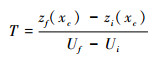
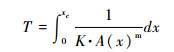
当裂点溯源迁移至河流源头,早期构造活动对河道的影响被“抹去”,新一期的构造活动完成了对整个河道的改造[32~33, 35~47]。裂点从流域出山口溯源迁移到河流源头所用的时间,称为地貌响应时间[20, 47~48]。假设初始时刻,河道处于与隆升速率Ui相平衡的状态,河流源头的高程为zi(xc)。当隆升速率改变为Uf,河道高程随之发生改变,当达到与Uf相平衡的状态时,河流源头的高程记作zf(xc)。那么,地貌响应时间(以T表示)为[37]:
|
(21) |
其中,xc为河流出水口到河流源头的溯源距离。以河流出水口作为参考点,则其相对高程为0。根据公式(6)所示的χ-z变换表达河道源头的高程,则地貌响应时间为[10, 45~48]:
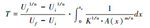
|
(22) |
对于线性情况(n=1),地貌响应时间可以简化为:
|
(23) |
公式(22)也被应用与求解线性的瞬态方程[28, 32~33, 44]。比较公式(22)与(23),可以发现:虽然河道高程剖面的重塑与构造活动有着密切联系,对于非线性条件,地貌响应时间与隆升速率密切相关;而对于线性情况,地貌响应时间仅取决于侵蚀系数和汇水面积,与隆升速率并无显著联系。
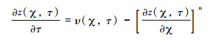
3 水力侵蚀瞬态方程的解如公式(1)所示的水力侵蚀方程中含有大量的未知参数,而侵蚀系数K也比较难于确定。因此,在求解方程时首先需要利用一些数学变换,减少参数个数,消除K对方程计算结果的影响。令τ=K·A0m·t,υ=U(x,t)/(K·A0m),这样时间项和速度项都变成了无维度的项了。则方程(1)的形式可以转化为[32]:
|
(24) |
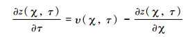
当河道侵蚀速率与河道坡度之间存在线性关系时(n=1),河道裂点不存在“被吞并”的现象[32]。因而,河道纵剖面可以完整地记录区域基岩隆升历史。此时,方程(24)可以简化为[32]:
|
(25) |
Goren等[33]求得该方程的解析解:
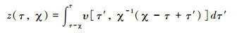
|
(26) |
线性方程的解析解(公式(26))将河道高程剖面的演化过程以连续的数学函数表示,从中也可以得到现今河道高程与隆升速率的时空分布特征的关系(公式27):
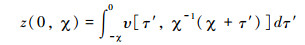
|
(27) |
假设流域基岩隆升速率在空间上分布均匀,则河道现今高程可以表示为[33]:
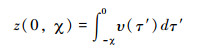
|
(28) |
将河道纵剖面分割成一系列节点,将公式(28)进行离散化:
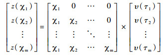
|
(29) |
这样,公式(28)就被转化为一个线性方程组。通过现今河道高程,求解这个离散的方程组,则隆升历史可以通过求出。需要指出的是,此时求得的是无维度的υ,需要借助于变换[33]U(x,t)=υ×(K·A0m)得到实际的隆升速率。
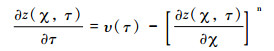
3.2 非线性瞬态方程求解对于非线性情况则比较复杂。Royden和Perron[32]假设隆升速率仅随时间变化,则公式(24)可以简化为:
|
(30) |
该方程的解析解:
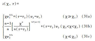
|
其中:

|
(32) |
本文主要介绍公式(31)和(32)的物理意义(非线性方程求解过程十分复杂,本文不作详细推导)。τ2为隆升速率变化的时间节点。在τ2之前,区域隆升速率为υ1;在τ2之后,区域隆升速率为υ2。
当隆升速率由υ1变化为υ2,河流流经区域经历了两次构造隆升,河道高程剖面上保留了两次构造活动的影响[32]。如图 4a所示,在时间节点τ2以前,隆升速率为υ1,其对河道的影响残留在χ1以上位置。换言之,在河道χ-z plot上横坐标大于χ1的部分,保持与早期隆升相平衡的状态(公式(31a))。在时间节点τ2以后,隆升速率为υ2。在河道χ-z plot上横坐标小于χ2的部分,保持与新一期隆升相平衡的状态(公式(31c))。图 4a中,n > 1且υ1 > υ2,由公式(32)可知χ1 > χ2。在χ1和χ2之间,河道虽然不受早期隆升事件的影响,但也尚未达到与新的隆升速率相平衡的状态。这一段弯曲的部分,函数表达如公式(31b),称为Stretch zone。如果后期加速隆升υ2 > υ1,则χ2 > χ1,表明后期构造活动会影响前期稳态的河道,早期构造活动对河道的影响会被部分抹掉。此时,河道χ-z plot不会出现弯曲段,而会出现一个很明显的裂点,称为consuming knickpoint(图 4b)。

|
图 4 不同参数(n和隆升历史)条件下河道χ-z plot的形态特征(据文献[32]修改) Fig. 4 The shape of χ-z plot based on different n value and rock uplift history, modified from reference[32] |
而n < 1的情况则相反。如果υ1 > υ2,这样χ1 < χ2,后期构造活动会部分抹掉早期构造活动对河道的影响,河道上出现consuming knickpoint(图 4c);而当υ1 < υ2,这样χ1 > χ2,后期构造活动不会对前期稳态的河道产生影响,χ1与χ2之间出现stretch zone(图 4d)。
因此,可以通过χ-z plot的形态大致判别n的取值范围。例如,已知某流域后期隆升速率高(河道下游河段χ-z plot的斜率大),如果河道出现stretch zone则n < 1,如果河道出现明显裂点(consuming knickpoint),则n > 1。
4 实例研究 4.1 线性非稳态方程应用实例——南美洲安第斯高原Cotahuasi河如图 5所示,Cotahuasi河位于秘鲁境内,从南美洲安第斯高原北部向南流入太平洋经。河流全长约300 km,河道总体落差超过6000 m。Cotahuasi河切穿安第斯高原西部边界,形成南美洲最深的峡谷——Cotahuasi-Ocoña大峡谷,峡谷落差超过3000 m[28]。热年代学研究揭示出Cotahuasi河下切始于13~10 Ma[49],这通常被认为是高原隆升最晚发生的时间[50]。Fox等[28]利用水力侵蚀方程(线性瞬态形式)和Cotahuasi流域内所有河道高程剖面,模拟了高原隆升历史。

|
图 5 Cotahuasi流域位置及水系分布(据文献[28]修改) Fig. 5 The location of drainage Cotahuasi and the distribution of streams, modified from reference[28] |
Fox等[28]提取了流域内所有的河流水系(流域面积临界值设置为1 km2),水系分布如图 5。根据参考凹度值0.35,计算得到所有河流的χ-z plot(图 6a)。可以很明显地看出来,在χ值约为50 m和80 m的地方,χ-z plot存在拐点。这说明该流域的隆升历史比较复杂,至少存在两次隆升速率的突变。利用线性方程组(公式(29))模拟区域隆升历史,可以发现时间节点τ超过100 m的部分,无维度的隆升速率υ一直保持着约为10的低值;时间节点τ从100 m到80 m的部分,υ迅速增加到约60;时间节点τ从80 m到50 m的部分,υ则保持不变;当τ从50 m开始,υ突然降低到30。

|
图 6 Cotahuasi流域所有水系的χ-z plot (a)和据此模拟的高原隆升历史(b)(据文献[28]修改) Fig. 6 The χ-z plots of all the streams of drainage Cotahuasi (a) and the derived rock uplift history of the Andean Plateau, modified from reference[28] |
需要指出的是,经过变换后得到的时间τ单位是m,与χ值单位相同。利用侵蚀系数K=4 m0.3/Ma(其中0.3=1-(2×0.35),0.35是流域参考凹度;m0.3/Ma整体作为侵蚀系数K的单位)校准τ和无维度的隆升速率υ,可以得到实际的隆升历史:安第斯高原北部在约30 Ma之前,隆升速率一直保持在约0.03 km/Ma的低值状态;而从30 Ma开始,仅用了不到10 Ma的时间,隆升速率就突增到0.20~0.25 km/Ma,而后一直保持不变;但从约12 Ma开始,隆升速率陡降到0.13 km/Ma。模拟结果说明,安第斯高原北部在20~13 Ma之间,存在脉冲式的隆升[28]。
在模拟隆升历史时候需要对河道χ-z plot中的χ值进行划分,这涉及到分割点的优化运算,超出了本文的讨论范畴。图 6b所示的模拟结果是Fox等[28]中最佳的拟合结果,并不是他们模拟工作的全部。Fox等[28]利用MCMC方法[51](Markov Chain Monte Carlo,马尔科夫链蒙特卡洛)寻找河道χ-z plot中的时间节点,然后根据一系列选择结果得到不同的隆升历史及其对应的后验概率,最后从中选择概率最大(即最佳)的结果。关于节点分割的优化方法,本文不作详细深入的探讨。
4.2 非线性方程应用实例——意大利半岛Rio Torto河Rio Torto河位于意大利中部,穿过Fiamignano正断层(图 7)。断层活动导致河道产生裂点并溯源迁移,因此,Fiamignano断裂的垂向滑动控制着Rio Torto河上游流域的演化[32](这里的河流上游是指位于Fiamignano断层上升盘的流域)。上游流域盆地面积约65 km2,高程从1865 m下降至569 m,盆地整体起伏约1300 m。但是,对于Rio Torto河干流而言,河道落差约600 m,远小于流域盆地的整体落差(图 8a)。

|
图 7 Rio Torto流域位置及其干流 Fig. 7 Location of drainage Rio Torto and its main stream |

|
图 8 Rio Torto流域干流的河流高程剖面(a)和χ-z plot (b)(据文献[32]修改) 图b中,蓝色实线为河道χ-z plot;设定参数n=0.5,τ2=850,υ1=0.2,υ2=0.7,模拟河道χ-z plot;早期隆升速率υ=0.2形成的稳态河道如深灰色实线标记,后期隆升速率υ=0.7形成的稳态河道如黑色实线标记,浅灰色曲线表示响应后期隆升但未达到稳态的河道的χ-z plot Fig. 8 The longitude profile of the main stream of drainage Rio Torto (a) and its χ-z plot (b). In Fig (b), parameters are:n=0.5, τ2=850, υ1=0.2, υ2=0.7. The dark gray line show a steady-state river profile under υ1=0.2, the black line show a steady-state river profile under υ2=0.7, the light gray curve shows a transient river segment under υ2=0.7(modified from reference[32]) |
自3 Ma以来,Fiamignano断层的垂向滑动速率一直保持在0.30 mm/a左右,而在约0.75 Ma以来,断层滑动速率突增到1.0 mm/a[52~53]。在这样的构造背景下,Rio Torto河干流的上游部分被分为了三段:相对海拔约500 m以上河段,处于均衡状态,陡峭系数偏低;相对海拔约300 m以下河段,处于均衡状态,陡峭系数高;而在两者之间,存在弯曲的χ-z plot(图 8b)。
Royden和Perron[32]设定参数:n=0.5,τ2=850,υ1=0.2,υ2=0.7。即:在时间节点为850的时候,断层滑动速率发生显著改变。早期,在无维度的隆升速率υ1=0.2条件下,形成了均衡的河道,这部分河道现今残留在流域高海拔区域(图 8b中深灰色直线表示);后期,υ2=0.7条件下,形成了均衡的河道,这部分河道在流域低海拔区域(图 8b中黑色直线表示);而当隆升速率由0.2向0.7突变的过程中(相对于3 Ma而言,这一时间段非常短暂),河道虽然响应新的隆升速率,但尚未达到均衡状态(图 8b中浅灰色曲线表示)。
图 8b中拟合的河道χ-z plot是经过了大量参数选择之后得到的最优模拟结果。无维度隆升速率0.2 mm/a和0.7 mm/a,比例为0.35,非常接近于实际的隆升速率比率0.33(早期隆升速率0.3 mm/a,后期隆升速率1.0 mm/a)。图 8b所示的拟合结果也与实际河道的χ-z plot极为吻合,这说明实例中利用水力侵蚀方程,从河流高程剖面中提取区域隆升速率信息,模拟区域的隆升历史是较为成功的。
5 结论本文重点介绍了应用水力侵蚀瞬态方程研究非均衡河道高程剖面的相关进展。这方面的研究主要包含两个方面:裂点溯源迁移和隆升历史模拟。这两方面是相辅相成的。一般而言,非均衡河道的标志是河道出现明显的裂点。裂点的出现,与区域构造活动相关;裂点溯源迁移,表示构造活动对水系河道的改造;裂点到达河流源头,标志着以此构造活动完成了对河道整体的改造,同时也意味着早期的构造活动痕迹被磨灭。因此,研究裂点的运动特征,对于模拟区域隆升历史相当重要。
当河流侵蚀速率与河道坡度线性相关(满足线性条件),不同时期构造活动产生的裂点以均匀的水平速率溯源迁移。那么,裂点在溯源迁移过程中,只要尚未到达河流源头,早期生成的裂点就不会被后期生成的裂点“吞并”,也就是说不存在构造信息缺失。而对于非线性情况,裂点溯源迁移速率不等,早期生成的裂点可能被后期生成的裂点“吞并”,河道高程剖面可能保存不了完整的区域隆升历史信息。所以,模拟区域隆升历史,必须要通过实际研究,判别研究区域是否满足线性条件;对于非线性情况,要深入研究裂点溯源迁移规律。
对于求解方程,采用χ值变换的方法,假设区域隆升速率仅随时间变化,求得方程的解析解,从而模拟区域隆升历史。对于线性方程而言,需要划分χ值空间以得到离散的线性方程组,求得各个时间段的隆升速率。而非线性情况则相对复杂,需要根据河道χ-z plot的形态(是否存在stretch zone或者consuming knickpoint)判别坡度指数n的大小,然后选择一系列参数(隆升速率及其变化的时间节点),根据非线性方程的解析解拟合河道χ-z plot,最后寻找拟合程度最佳的参数,得到区域隆升历史。而对于区域隆升速率随时间、空间都发生变化,并且n≠1的情况,方程的解析解尚未被求出。这应当是今后该领域进一步的发展方向。
致谢 匿名审稿专家提出的宝贵意见对于本文的提高大有裨益;编辑杨美芳老师对文章的完善付出辛勤劳动。笔者在此一并致以谢意。
| 1 |
Korup O, Montgomery D R. Tibetan Plateau river incision inhibited by glacial stabilization of the Tsangpo Gorge. Nature, 2008, 455: 786-790. DOI:10.1038/nature07322 |
| 2 |
Wang P, Scherler D, Liu-Zeng J et al. Tectonic control of Yarlung Tsangpo Gorge revealed by a buried canyon in southern Tibet. Science, 2014, 346(6212): 978-981. DOI:10.1126/science.1259041 |
| 3 |
Fox M, Leith K, Bodin T et al. Rate of fluvial incision in the Central Alps constrained through joint inversion of detrital 10Be and thermochronometric data. Earth and Planetary Science Letters, 2015, 411: 27-36. DOI:10.1016/j.epsl.2014.11.038 |
| 4 |
Pan Baotian, Geng Haopeng, Hu Xiaofei et al. The topographic controls on the decadal-scale erosion rates in Qilian Shan Mountains, N.W. China. Earth and Planetary Science Letters, 2010, 292(1-2): 148-157. DOI:10.1016/j.epsl.2010.01.030 |
| 5 |
Korup O, Schlunegger F. Bedrock landsliding, river incision, and transience of geomorphic hillslope-channel coupling:Evidence from inner gorges in the Swiss Alps. Journal of Geophysical Research, 2007, 112(F03027): 1-19. DOI:10.1029/2006JF000710 |
| 6 |
Flint J J. Stream gradient as a function of order, magnitude, and discharge. Water Resources Research, 1974, 10(5): 969-973. DOI:10.1029/WR010i005p00969 |
| 7 |
Howard A D, Kerby G. Channel changes in badlands. Geological Society of America Bulletin, 1983, 94(6): 739-752. DOI:10.1130/0016-7606(1983)94<739:CCIB>2.0.CO;2 |
| 8 |
Whipple K X, Tucker G E. Dynamics of the stream-power river incision model:Implications for height limits of mountain ranges, landscape response timescales, and research needs. Journal of Geophysical Research, 1999, 104(17): 17661-17674. |
| 9 |
李小强, 任金卫, 杨攀新等. 六盘山东西两侧第四纪以来构造差异隆升速率递变性. 第四纪研究, 2015, 35(2): 445-452. Li Xiaoqiang, Ren Jinwei, Yang Panxin et al. Regularity of tectonic differential uplifting rates of both the east and west sides of Liupanshan Mountain since the Quaternary. Quaternary Sciences, 2015, 35(2): 445-452. DOI:10.11928/j.issn.1001-7410.2015.02.19 |
| 10 |
Snyder N P, Whipple K X, Tucker G E et al. Landscape response to tectonic forcing:Digital elevation model analysis of stream profiles in the Mendocino triple junction region, northern California. Geological Society of America Bulletin, 2000, 112(8): 1250-1263. DOI:10.1130/0016-7606(2000)112<1250:LRTTFD>2.0.CO;2 |
| 11 |
胡小飞, 潘保田, Kirby E等. 河道陡峭指数所反映的祁连山北翼抬升速率的东西差异. 科学通报, 2010, 55(23): 3205-3214. Hu Xiaofei, Pan Baotian, Kirby E et al. Spatial differences in rock uplift rates inferred from channel steepness indices along the northern flank of the Qilian Mountain, northeast Tibetan Plateau. Chinese Science Bulletin, 2010, 55(23): 3205-3214. |
| 12 |
李琼, 潘保田, 高红山等. 祁连山东段基岩河道宽度对差异性构造抬升的响应. 第四纪研究, 2015, 35(2): 453-464. Li Qiong, Pan Baotian, Gao Hongshan et al. Bedrock channel width responses to differential tectonic uplift in eastern Qilian Mountain. Quaternary Sciences, 2015, 35(2): 453-464. DOI:10.11928/j.issn.1001-7410.2015.02.20 |
| 13 |
王军, 李小强, 贾科等. 阿尔金山东段河道陡峭指数对区域隆升差异的响应. 第四纪研究, 2017, 37(2): 260-270. Wang Jun, Li Xiaoqiang, Jia Ke et al. The response of the Channel steepness index to the difference of uplift rate in the eastern section of Altyn Mountains. Quaternary Sciences, 2017, 37(2): 260-270. |
| 14 |
Tarboton D G, Bras R L, Rodriguez-Iturbe I. Scaling and elevation in river networks. Water Resources Research, 1989, 25: 2037-2051. DOI:10.1029/WR025i009p02037 |
| 15 |
Kirby E, Whipple K X, Tang W et al. Distribution of active rock uplift along the eastern margin of the Tibetan Plateau:Inferences from bedrock river profiles. Journal of Geophysical Research, 2003, 108(B4): 2217-2240. |
| 16 |
Wobus C, Whipple K X, Kirby E et al. Tectonics from topography:Procedures, promise, and pitfalls. Geological Society of America Special Paper, 2006, 398(12): 55-74. |
| 17 |
Perron J T, Royden L. An integral approach to bedrock river profile analysis. Earth Surface Process and Landforms, 2013, 38: 570-576. DOI:10.1002/esp.3302 |
| 18 |
李小强, 王军, 熊仁伟等. 六盘山地区河道陡峭指数对隆升速率差异的响应. 第四纪研究, 2016, 36(2): 443-452. Li Xiaoqiang, Wang Jun, Xiong Renwei et al. The response of the channel steepness index to the difference of uplift rate in the Liupanshan Mountain area. Quaternary Sciences, 2016, 36(2): 443-452. |
| 19 |
刘兴旺, 袁道阳, 吴赵等. 六盘山断裂带活动性差异及其对六盘山隆升的影响. 第四纪研究, 2016, 36(4): 898-906. Liu Xingwang, Yuan Daoyang, Wu Zhao et al. Differetial activeties along the Liupanshan Mountain fault zone and its influence on uplift of the Liupanshan Mountain. Quaternary Sciences, 2016, 36(4): 898-906. |
| 20 |
秦翔, 施炜, 李恒强等. 基于DEM地形特征因子的青藏高原东北缘宁南弧形断裂带活动性分析. 第四纪研究, 2017, 37(2): 213-223. Qin Xiang, Shi Wei, Li Hengqiang et al. Tectonic differences of the Southern Ningxia arc-shape faults in the northeast Tibetan Plateau based on Digital Elevation Model. Quaternary Sciences, 2017, 37(2): 213-223. |
| 21 |
刘蓓蓓, 崔之久, 刘耕年等. 基于面积-高程积分法的岷山雪宝顶-九寨沟地貌形态分析. 第四纪研究, 2017, 37(2): 224-233. Liu Beibei, Cui Zhijiu, Liu Gengnian et al. Geomorphologic analysis of the Xuebaoding-Jiuzhaigou area in Min Shan based on Hypsometric Integral method. Quaternary Sciences, 2017, 37(2): 224-233. |
| 22 |
杜国云. 基于DEM的莱州湾南岸典型水系河间地提取及区域地貌演化研究. 第四纪研究, 2015, 35(2): 475-483. Du Guoyun. Interfluves extract based on DEM and Holocene development of geomorphology for the typical rivers in the south coast of the Laizhou Bay. Quaternary Sciences, 2015, 35(2): 475-483. DOI:10.11928/j.issn.1001-7410.2015.02.22 |
| 23 |
张沛全, 左天惠, 周青云等. 南盘江上游河网纵剖面图像及其构造指示意义. 第四纪研究, 2016, 36(2): 464-473. Zhang Peiquan, Zuo Tianhui, Zhou Qingyun et al. The drainage network and longitudinal profile image (DNLPI) of Nanpangjiang River upstream catchment and its tectonic implication. Quaternary Sciences, 2016, 36(2): 464-473. |
| 24 |
张会平, 张培震, 吴庆龙等. 循化-贵德地区黄河水系河流纵剖面形态特征及其构造意义. 第四纪研究, 2008, 28(2): 299-309. Zhang Huiping, Zhang Peizhen, Wu Qinglong et al. Characteristics of the Huanghe River longitudinal profiles around Xunhua-Guide area(NE Tibet) and their tectonics significance. Quaternary Sciences, 2008, 28(2): 299-309. |
| 25 |
Whipple K X, Hancock G S, Anderson R S. River incision into bedrock:Mechanics and relative efficacy of plucking, abrasion, and cavitation. Geological Society of America Bulletin, 2000, 112(3): 490-503. DOI:10.1130/0016-7606(2000)112<490:RIIBMA>2.0.CO;2 |
| 26 |
Berlin M M, Anderson R S. Modeling of knickpoint retreat on the Roan Plateau, Western Colorado. Journal of Geophysical Research, 2007, 112(F3): 1-16. |
| 27 |
Howard A D, Dietrich W E, Seidl M A. Modeling fluvial erosion on regional to continental scales. Journal of Geophysical Research:Earth Surface, 1994, 99(B7): 13971-13986. DOI:10.1029/94JB00744 |
| 28 |
Fox M, Bodin T, Shuster D L. Abrupt changes in the rate of Andean Plateau uplift from reversible jump Markov Chain Monte Carlo inversion of river profiles. Geomorphology, 2015, 238: 1-14. DOI:10.1016/j.geomorph.2015.02.022 |
| 29 |
Gallen S F, Wegmann K W. River profile response to normal fault growth and linkage:An example from the Hellenic forearc of south-central Crete, Greece. Earth Surface Dynamics, 2017, 5: 161-186. DOI:10.5194/esurf-5-161-2017 |
| 30 |
王一舟, 张会平, 郑德文等. 基岩河道河流水力侵蚀模型及其应用:兼论青藏高原基岩河道研究的迫切性. 第四纪研究, 2016, 36(4): 884-897. Wang Yizhou, Zhang Huiping, Zheng Dewen et al. Stream power incision model and its implications:Discussion on the urgency of studying bedrock channel across the Tibetan Plateau. Quaternary Sciences, 2016, 36(4): 884-897. |
| 31 |
李雪梅, 张会平. 河流瞬时地貌:特征、过程及其构造-气候相互作用内涵. 第四纪研究, 2017, 37(2): 416-430. Li Xuemei, Zhang Huiping. Transient fluvial landscape:Features, processes and its implication for tectonic-climate interaction. Quaternary Sciences, 2017, 37(2): 416-430. |
| 32 |
Royden L, Perron J T. Solutions of the stream power equation and application to the evolution of river longitudinal profiles. Journal of Geophysical Research:Earth Surface, 2013, 118(2): 497-518. DOI:10.1002/jgrf.20031 |
| 33 |
Goren L, Fox M, Willett S D. Tectonics from fluvial topography using formal linear inversion:Theory and applications to the Inyo Mountains, California. Journal of Geophysical Research:Earth Surface, 2014, 119: 1651-1681. DOI:10.1002/2014JF003079 |
| 34 |
Kirby E, Whipple K X. Quantifying differential rock-uplift rates via stream profile analysis. Geology, 2001, 29(5): 415-418. DOI:10.1130/0091-7613(2001)029<0415:QDRURV>2.0.CO;2 |
| 35 |
Wang Yizhou, Zhang Huiping, Zheng Dewen et al. Coupling slope-area analysis, integral approach and statistic tests to steady-state bedrock river profile analysis. Earth Surface Dynamics, 2017, 5: 145-160. DOI:10.5194/esurf-5-145-2017 |
| 36 |
Zhang H, Kirby E, Pitlick J et al. Characterizing the transient geomorphic response to base-level fall in the northeastern Tibetan Plateau. Journal of Geophysical Research:Earth Surface, 2017, 122(2): 546-572. DOI:10.1002/jgrf.v122.2 |
| 37 |
Neely A B, Bookhagen B, Burbank D W. An automated knickzone selection Algorithm (KZ-Picker) to analyze transient landscapes:Calibration and validation. Journal of Geophysical Research:Earth Surface, 2017, 122(2): 1236-1261. |
| 38 |
Kirby E, Whipple K X. Expression of active tectonics in erosional landscapes. Journal of Structural Geology, 2012, 44: 54-75. DOI:10.1016/j.jsg.2012.07.009 |
| 39 |
Regalla C, Kirby E, Fisher D et al. Active forearc shortening in Tohoku, Japan:Constraints on fault geometry from erosion rates and fluvial longitudinal profiles. Geomorphology, 2013, 195: 84-98. DOI:10.1016/j.geomorph.2013.04.029 |
| 40 |
Wang Yizhou, Zhang Huiping, Zheng Dewen et al. How a stationary knickpoint is sustained:New insights into the formation of the deep Yarlung Tsangpo Gorge. Geomorphology, 2017, 285: 28-43. DOI:10.1016/j.geomorph.2017.02.005 |
| 41 |
Harkins N, Kirby E, Heimsath A et al. Transient fluvial incision in the headwaters of the Yellow River, northeastern Tibet, China. Journal of Geophysical Research, 2007, 112: 1-21. DOI:10.1029/2006JF000570 |
| 42 |
Fox M, Goren L, May D A et al. Inversion of fluvial channels for paleorock uplift rate in Taiwan. Journal of Geophysical Research:Earth Surface, 2014, 119: 1853-1875. DOI:10.1002/2014JF003196 |
| 43 |
张会平, 张培震, 樊祺诚. 河流裂点的发育及其溯源迁移:以鸭绿江-望天鹅火山区为例. 中国科学:地球科学, 2011, 54(11): 1746-1753. Zhang Huiping, Zhang Peizhen, Fan Qicheng. Initiation and recession of the fluvial knickpoints:A case study from the Yalu River-Wangtian'e volcanic region, Northeastern China. Science China:Earth Sciences, 2011, 54(11): 1746-1753. |
| 44 |
Rudge J F, Roberts G G, White N J et al. Uplift histories of Africa and Australia from linear inverse modeling of drainage inventories. Journal of Geophysical Research:Earth Surface, 2015, 120: 894-914. DOI:10.1002/2014JF003297 |
| 45 |
Whipple K X. Bedrock rivers and the geomorphology of active orogens. Annual Review of Earth and Planetary Sciences, 2004, 32: 151-185. DOI:10.1146/annurev.earth.32.101802.120356 |
| 46 |
Rosenbloom N A, Anderson R S. Hillslope and channel evolution in a marine terraced landscape, Santa Cruz, California. Journal of Geophysical Research, 1994, 99(B7): 14013-14030. DOI:10.1029/94JB00048 |
| 47 |
Whipple K X. Fluvial landscape response time:How plausible is steady-state denudation?. American Journal of Science, 2001, 301(4-5): 313-325. DOI:10.2475/ajs.301.4-5.313 |
| 48 |
Snyder N P, Whipple K X, Tucker G E. Channel response to tectonic forcing:Field analysis of stream morphology and hydrology in the Mendocino triple junction region, northern California. Geomorphology, 2003, 53: 97-127. DOI:10.1016/S0169-555X(02)00349-5 |
| 49 |
Schildgen T F, Ehlers T A, Whipp D M et al. Quantifying canyon incision and Andean Plateau surface uplift, southwest Peru:A thermochronometer and numerical modeling approach. Journal of Geophysical Research:Earth Surface, 2009, 114(F4). DOI:10.1029/2009JF001305 |
| 50 |
Schildgen T F, Balco G, Shuster D L. Canyon incision and knickpoint propagation recorded by apatite 4He/3He thermochronometry. Earth and Planetary Science Letters, 2010, 293(3): 377-387. |
| 51 |
Gallagher K, Charvin K, Nielsen S et al. Markov Chain Monte Carlo (MCMC) sampling methods to determine optimal models, model resolution and model choice for Earth science problems. Marine & Petroleum Geology, 2009, 26(4): 525-535. |
| 52 |
Whittaker A C, Cowie P A, Attal M et al. Bedrock channel adjustment to tectonic forcing:Implications for predicting river incision rates. Geology, 2007, 35(2): 103-106. DOI:10.1130/G23106A.1 |
| 53 |
Whittaker A C, Cowie P A, Attal M et al. Contrasting transient and steady-state rivers crossing active normal faults:Newfield observations from the central Apennines, Italy. Basin Research, 2007, 19(4): 529-556. DOI:10.1111/bre.2007.19.issue-4 |
Abstract
The landscape evolution of active orogens can be regarded as the coupling between climatic change and tectonic movement. Rivers originating from and flowing through orogens have been affected and reshaped by regional rock uplift and deformation. The related tectonic signals, as a result, can be recorded and stored in stream longitudinal profiles. The stream-power river incision model, combing bedrock uplift, river incision, and topographic evolution, makes it possible to extract the spatial and temporary details of rock uplift. The well known stream-power river incision model is expressed as a non-linear partial differential equation (PDE), in which the temporal variation of bedrock channel elevation is the competition between rock uplift and channel incision. During the past 40 years, studies had been on its steady-state form. Assuming that the river profile is under a steady state with spatially invariant rock uplift, a power-law scaling between channel slope and drainage area can be derived. Then, a steepness index is yielded to quantify the spatial pattern of rock uplift rates. However, the landforms in active orogens are usually in a transient state where rock uplift cannot be balanced by river incision. With the development of mathematics and computer science, more and more scholars have been working on the solutions (both analytical and numerical)of the transient PDE. Based on the stream power incision model (allowing both spatially and temporarily variant rock uplift and a non-linear relationship between river incision and channel gradient), the velocity of knickpoint migration was derived. Then, the landscape response time could be calculated by dividing the river length by the horizontal velocity of knickpoint migration. Both knickpoint migration velocity and landscape time vary a lot between linear and non-linear conditions. For the linear condition, knickpoints migrate upstream in the same horizontal velocity that depends on erodibility and drainage area. The landscape response time shows no relation with rock uplift rate. Thus, the "older" knickpoints cannot be erased by "younger" ones, leaving a full rock uplift history. To model the rock uplift history, the χ-z plot is divided into a series of segments. Each segment can be regarded as a normalized time interval and elevation difference. By dividing the elevation difference by time interval, we can get the transformed rock uplift rate at the specified time. While for the non-linear condition, the horizontal velocities of knickpoints migrating upstream vary largely. Those "older" knickpoints might be erased by "younger" ones. The landscape response time depends on the rock uplift rates before and after the tectonic event. Therefore, some details of rock uplift will be lost owing to the non-uniform velocities. Assuming spatially invariant rock uplift, the analytical solution to the PDE was derived. For two conditions (n < 1, rock uplift rate increases, or n > 1, rock uplift rate decreases), a full rock uplift history will be stored and a "stretch zone" was present along the χ-z plot. When n > 1, rock uplift rate decreases, or n < 1, rock uplift rate increases, the "slope patch" generated elder will be partly eased, resulting into a "consuming knickpoint". However, spatial information from the non-linear transient equation is still confusing.