 2013, Vol. 1
The article information
- Liu-Ming Yan, Chao Sun, Hui-Ting Liu
- Opposite phenomenon to the flying ice cube in molecular dynamics simulations of flexible TIP3P water
- Advances in Manufacturing, 2013, 1(2): 160–165
- http://dx.doi.org/10.1007/s40436-013-0024-3
-
Article history
- Received: 2013-04-17
- Accepted: 2013-04-28
- Published online: 2013-06-14


The equipartition theorem, the overall energy of a system is equally shared among its various degrees of freedom on average when thermal equilibrium reaches, is one of the most definite and important results of classical statistical mechanics. And it has been successfully applied to estimate heat capacities of gases, liquids, and solids, to relate the temperature of a system to its average kinetic energies, and even to estimate stellar temperatures [1]. The generalized equipartition theorem requires that the Hamiltonian diverges at the upper/lower bounds of the corresponding variable of interest [2]. Although the equipartition theorem was formulated in the 19th century, it still attracts great research interest from physics, chemistry, and stellar physics [3, 4, 5, 6, 7, 8, 9, 10, 11, 12].
The molecular dynamics (MD) simulation, as an uncompensated research tool to the theoretical methods and experimental methods, is playing an increasingly important role in the study of complicated molecular systems in the field of chemistry, biology, physics, and materials science [13]. However, the numerical errors inherited from the calculation of the intermolecular and intramolecular forces, from the integration of equations of motions, and from the scaling of velocities and cell size to maintain constant pressure and constant temperature may cause erroneous results [14]. During the force calculations, errors are inherited from the numerical rounding and the long distance cutoff. The numerical rounding errors are usually insignificant, and special treatment is not needed in most simulations. The long distance cutoff error is similar to the situation where the original force field model is substituted with a force field model truncated at cutoff distance [13]. Since force field models are only approximate to the real world molecule, a truncated force field model actually affects only the effectiveness of force field model, but not the effectiveness of the MD simulation method. The numerical errors which are inherited from the integration of equations of motion cause the great problem. If an unsuitable integration scheme is applied, or unsuitable parameters are chosen, the calculated trajectory may deviate greatly from the accurate trajectory, and erroneousness results may be obtained [14]. For example, the numerical errors may cause the so-called flying ice cube phenomenon where high frequency vibrational kinetic energy is continuously converted to the low frequency translational motion and rotational motion when certain type of scaling algorithm is used [15].
The velocity distribution function of molecules represents another important issue that should be concerned in MD simulation. It is well known that the digitalized system trajectory, which is generated by the numerical integration of the equations of motion during the MD simulation, represents an approximation to the real world trajectory. If the ergodic hypothesis or quasi-ergodic hypothesis is satisfied, the time averages of properties along the approximated digitalized trajectory will converge to the ensemble averages [13]. On the other hand, if the ergodic hypothesis is not satisfied, the time averages of properties along the approximated digitalized trajectory may deviate from the ensemble averages and misrepresent the system. An examination of the agreement between the velocity distribution function calculated from MD simulation and the Maxwell-Boltzmann distribution function may verify if the ergodic hypothesis satisfies since the velocity distribution function of an ergodic molecular system will relax into Maxwell-Boltzmann distribution [16].
In this work, we study the motion of the flexible (or rigid) TIP3P water using MD simulation, and project the overall kinetic energy onto translational motion, rotational motion, and vibrational motion (for the flexible TIP3P water only). We also evaluate the velocity distribution function of the translational motion, of the oxygen atoms motion, and of the hydrogen atoms motion. From these simulations, an opposite phenomenon to the flying ice cube where kinetic energy is drained from the high frequency vibrational motion to the low frequency translational motion and rotational motion is reported. 2 Simulation methods 2.1 Molecular model of water
As an example, we simulate 1, 000 water molecules using MD simulation. Two types of force field models including the rigid TIP3P water model [17] and the flexible TIP3P water model are applied to the water molecules, respectively. The flexible TIP3P water model is based on the rigid TIP3P model with harmonic O-H bond and H-O-H bond angle [18, 19, 20]. The force field constant for O-H bond stretching is 4.63 MJ mol-1 Å-2 and the equilibrium bond length is 0.9572 Å. The force field constant for the H-O-H bond angle is 837.36 kJ mol-1 rad-2, and the equilibrium bond angle is 104.52°. Although there are many other force field models for water molecule [21], our purposed of this work is to demonstrate if the equipartition theorem is applicable in MD simulation. Therefore, it will not loss generality which specific force field model is applied. 2.2 Evaluation of velocity distribution functions
Various velocity distribution functions corresponding to the translational motion, motion of the oxygen and hydrogen are generated from the recorded trajectory files. These velocity distribution functions are then fitted to the Maxwell-Boltzmann distribution function,

All the MD simulations are carried out using the DL_POLY program within the NPT ensemble [22]. Constant temperature and pressure are maintained by coupling to a bath (relaxation time 0.1 ps, pressure 101.325 kPa, temperature 300 K), following the Nosé-Hoover algorithm [23, 24]. Neighbor lists are recorded and updated per 10 steps with a primary cutoff distance of 8.5 Å and a shell width of 1 Å . The Lennard-Jones interaction is cutoff at 9.5 Å , and the Ewald summation algorithm at precision of 10-8 is applied to the calculation of electrostatic potential in account for long-range coulombic interaction. The leapfrog scheme is used in the integration of the equations of motion with a step time from 0.1 to 3.0 fs [25]. Both the Shake tolerance and quaternion tolerance are set to 10-8.
During the simulations, 5, 000, 000 time steps are run in the first period to ensure that the system reaches equilibrium. Then 1, 000, 000 production steps are carried out, and snapshots of the coordinates and velocities of all atoms of the last 200, 000 production steps are recorded per 10 steps in a trajectory file. The recorded trajectory file is then used to evaluate the kinetic energy in various motions, as well as the various velocity distribution functions. We also test the temperatures and velocity distribution functions from the trajectory file composed of 40, 000 snapshots and find no significant difference between these two methods. 3 Results and discussions 3.1 Case one: the flexible water system
In this work, it will focus on the effect of numerical errors inherited from the integration scheme, especially the choice of integration step time. In order to study the impact of the numerical errors on the kinetic energy distribution among the translational motion, the rotational motion, and the vibrational motion, the integration step time is varied at 0.1, to 0.3 and 0.6 fs. In Fig. 1, it shows the evolution of kinetic energies in the translational motion, rotational motion, and vibrational motion of the flexible TIP3P water. It could be seen that the translational motion and rotational motion usually share the same kinetic energy on average. However, the vibrational motion usually does not share the same kinetic energy as that of the translational motion or rotational motion. When the integration step time is small, at 0.1 fs or 0.3 fs, for example, the average kinetic energy of translational motion and rotational motion are at about 306 K, however, the vibrational energy is only 283 K (see Table 1).
 |
| Fig. 1 Evolution of temperature in translational motion (black), rotational motion (red), and vibrational motion (blue) for step time of: a 0.1 fs, b 0.3 fs, and c 0.6 fs. The rotational temperature and vibrational temperature have been shifted up 100 and 200 K to avoid the superposition of the evolution curves, respectively. The dotted green lines are guides to the eyes for temperatures predicted by the equipartition theorem. Flexible TIP3P model, NPT ensemble, the Nosé-Hoover algorithm (barostat 101.325 kPa, thermostat at 300 K, relaxation time 0.1 ps) |
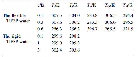 |
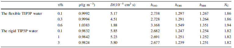
When the integration step time increases to 0.6 fs, an opposite phenomenon is observed. The kinetic energy of low frequency translational motion or rotational motion is lower than that of high frequency vibrational motion or the kinetic energies of the low frequency translational motion, and rotational motion are converted to the high frequency vibrational motion. In addition, the self-diffusion coefficient decreases as the step time increases as a direct result of the loss of the translational kinetic energy (see Table 2).
 |
Although the equipartition theorem is not universally applicable to the flexible TIP3P water, all the velocity distribution functions, which include the translational motion, the motion of oxygen, the motion of hydrogen, still agree with the Maxwell-Boltzmann distribution function (see Fig. 2). In addition, the temperature estimated from least square fit to the Maxwell-Boltzmann distribution also agrees well with what is calculated from the corresponding average kinetic energy of the molecules or the atoms.
The radial distribution functions do not seem to change significantly when the integration step time increases from 0.1 fs to 0.6 fs (see Fig. 3). However, as the integration step time increases, the first peak heights of the radial distribution functions and the coordination number (NC) or the number of hydrogen bonds formed increase (see Table 2). Meanwhile, the density of the simulated system also increases.
 |
| Fig. 2 Velocity distribution functions for the translational motion (red), the oxygen atoms (blue), and hydrogen atoms (green). The corresponding curves are best fits to the Maxwell-Boltzmann velocity distribution; and the inset is a magnification of part of the original picture. Flexible TIP3P model, NPT ensemble, the Nosé-Hoover algorithm (barostat 101.325 kPa, thermostat at 300 K, relaxation time 0.1 ps) |
 |
| Fig. 3 Radial distribution functions for the flexible TIP3P model, at 300 K, 101.325 kPa, NPT ensemble using the Nosé-Hoover algorithm, leapfrog algorithm integrated with step time 0.1 fs |
For comparison, we also simulate the water using the rigid TIP3P model. It is found that the equipartition theorem holds for rigid TIP3P water if the integration step time of 0.1, 1, or 3 fs is used. The kinetic energy of the rigid TIP3P water equally on average is distributed between the translational motion and the rotational motion within statistical error (see Fig. 4). The translational velocity distribution function agrees with the Maxwell-Boltzmann velocity distribution functions very well (see Fig. 5). From the translational temperature and rotational temperature which are listed in Table 1, it is concluded that the overall kinetic energy is equally partitioned into translational motion and rotational motion.
 |
| Fig. 4 Evolution of kinetic energy in translational motion (black) and rotational motion (red). In order to avoid the superposition of the evolution curves, the rotational kinetic energies have been shifted up 100 K. Step time: a 0.1, b 1.0, and c 3.0 fs. The dotted green lines are guides to the eyes for temperatures predicted by the equipartition theorem. RigidTIP3P water, NPTensemble, theNosé-Hoover algorithm (barostat 101.325 kPa, thermostat at 300 K, relaxation time 0.1 ps) |
 |
| Fig. 5 Velocity distribution function for the translational motion of rigid TIP3P water, NPT ensemble, the Nosé-Hoover algorithm (barostat 101.325 kPa, thermostat at 300 K, relaxation time 0.1 ps). The blue curve represents the best fit to the Maxwell-Boltzmann distribution |
The radial distribution functions (see Fig. 6) are similar to what has been reported in Ref. [21]. The density of simulated system varies from 0.9832, 0.9841, to 0.9824 g/cm3 as the integration step time varies from 0.1 fs, to 1 fs and 3 fs, in good agreement with each other and with reported value [21]. In Table 2, the simulated self-diffusion coefficients at 5.85 × 10⁻⁵, 5.23 × 10⁻⁵, 5.80 × 10⁻⁵ cm2/s for step time of 0.1, 1, and 3 fs, respectively, are also in good agreement with each other and with reported simulation results [21], however, exceed twice higher than the experimental value at ambient temperature of 2.310 × 10⁻⁵ cm2/s [26]. From these simulations, it could be concluded that the equipartition theorem is applicable for TIP3P rigid water model.
 |
| Fig. 6 Radial distribution functions g(r) for rigid TIP3P water. Simulated at 300 K, 101.325 kPa, NPT ensemble using the Nosé- Hoover algorithm, leapfrog algorithm, integration step time 1.0 fs |
The mechanism why the kinetic energy is drained from low frequency translational motion and rotational motion to high frequency vibrational motion is explained by the specific interaction between an oxygen atom and a hydrogen atom in flexible TIP3P model. The interatomic interaction between an oxygen atom and a hydrogen atom in the flexible water model includes a harmonic bond stretching force and an electrostatic attraction force (see Fig. 7). As a hydrogen atom approaches to the oxygen atom, it is firstly attracted by the oxygen atom, and then it is repelled as it goes closer than its equilibrium point. The repulsion region is between 0.45 and 0.84 Å . If the hydrogen atom goes very close to the oxygen atom, it will be attracted by the oxygen atom again. During the NPT ensemble MD simulation, the hydrogen atom is more probably gaining kinetic energy during the velocity scaling. As a result, the internal vibrational motion gains kinetic energy, and the translational motion and rotational motion loses kinetic energy.
 |
| Fig. 7 Interatomic interaction between an oxygen and hydrogen in flexible TIP3P water. Green the harmonic bond stretching potential; blue the sum of the harmonic bond stretching and electrostatic potential; red the overall interatomic force which is scaled by the mass of a hydrogen atom |
In conclusion, the integration step time has great impact on the MD simulation results for the flexible TIP3P water. If the integration step time is 0.3 fs or less, the flying ice phenomenon is observed as kinetic energy is drained from the high frequency vibrational motion to the low frequency translational motion and the rotational motion. The equipartition theorem is only applicable to the translational motion and rotational motion, but not to the vibrational motion. If the integration step time is 0.6 fs, an opposite phenomenon to the flying ice cube is observed as kinetic energy is drained from the low frequency translational motion and rotational motion to the high frequency vibrational motion. However, the equipartition theorem is still applicable to the translational motion and rotational motion, but not to the vibrational motion. For rigid TIP3P water, the equipartition theorem is applicable for integration step time up to 3 fs and the translational velocity distribution function obeys the Maxwell-Boltzmann distribution.
For the cases that the equipartition theorem is partly applicable, the translational velocity distribution function of flexible TIP3P waters agrees well with the Maxwell- Boltzmann distribution function. And the atomistic velocities of the oxygen atoms and hydrogen atoms also fit well to the Maxwell-Boltzmann distribution. Furthermore, the temperatures which are calculated by fitting the velocity distribution functions to the Maxwell-Boltzmann distribution functions are in good agreement with the temperatures evaluated directly from the average of molecular (or atomistic) kinetic energy.
Acknowledgments The authors thank the Laboratory for Microstructures, Shanghai University for carrying out the structural characterization, and acknowledge the financial support from the National Natural Science Foundation of China (Grant No. 21073118), the Innovation Program of Shanghai Municipal Education Commission (Grant No. 13ZZ078).| 1. | Chandrasekhar S (1939) An introduction to the study of stellar structure. University of Chicago Press, Chicago, pp 49-53 |
| 2. | Tolman RC (1918) A general theory of energy partition with applications to quantum theory. Phys Rev 11(4):261-275 |
| 3. | Martínez S, Pennini F, Plastino A et al (2002) On the equipartition and virial theorems. Phys A 305(1-2):48-51 |
| 4. | Plastino AR, Lima JAS (1999) Equipartition and virial theorems within general thermostatistical formalisms. Phys Lett A 260(1-2): 46-54 |
| 5. | Uline MJ, Siderius DW, Corti DS (2008) On the generalized equipartition theorem in molecular dynamics ensembles and the microcanonical thermodynamics of small systems. J Chem Phys 128(12):124301 |
| 6. | Schnack J (1998) Molecular dynamics investigations on a quantum system in a thermostat. Phys A 259(1-2):49-58 |
| 7. | Shirts RB, Burt SR, Johnson AM (2006) Periodic boundary condition induced breakdown of the equipartition principle and other kinetic effects of finite sample size in classical hard-sphere molecular dynamics simulation. J Chem Phys 125(16):164102 |
| 8. | Shirts RB, Shirts MR (2002) Deviations from the Boltzmann distribution in small microcanonical quantum systems: two approximate one-particle energy distributions. J Chem Phys 117(12): 5564-5575 |
| 9. | Bakunin OG (2005) Correlation effects and nonlocal velocity distribution functions. Phys A 346(3-4):284-294 |
| 10. | Keffer DJ, Baig C, Adhangale P et al (2008) A generalized Hamiltonian-based algorithm for rigorous equilibrium molecular dynamics simulation in the canonical ensemble. J Non-Newton Fluid Mech 152(1-3):129-139 |
| 11. | Campisi M (2005) On the mechanical foundations of thermodynamics: the generalized Helmholtz theorem. Stud Hist Philos Sci Part B 36(2):275-290 |
| 12. | Criado-Sancho M, Jou D, Casas-Vázquez J (2006) Nonequilibrium kinetic temperatures in flowing gases. Phys Lett A 350(5-6):339-341 |
| 13. | Allen MP, Tildesley DJ (1990) Computer simulation of liquids. Oxford University Press, Oxford |
| 14. | Frenkel D, Smit B (2002) Understanding molecular simulation: from algorithms to applications, 2nd edn. Academic Press, New York |
| 15. | Harvey SC, Tan RKZ, Cheatham TE III (1998) The flying ice cube: velocity rescaling in molecular dynamics leads to violation of energy equipartition. J Comput Chem 19(7):726-740 |
| 16. | Mohazzabi P, Helvey SL, McCumber J (2002) Maxwellian distribution in non-classical regime. Phys A 316(1-4):314-322 |
| 17. | Jorgensen WL, Chandrasekhar J, Madura JD et al (1983) Comparison of simple potential functions for simulating liquid water. J Chem Phys 79(2):926-935 |
| 18. | Liew CC, Inomata H, Arai K (1998) Flexible molecular models for molecular dynamics study of near and supercritical water. Fluid Phase Equilib 144(1-2):287-298 |
| 19. | Neria E, Fischer S, KarplusM(1996) Simulation of activation free energies in molecular systems. J Chem Phys 105(5):1902-1921 |
| 20. | Yan L, Zhu S, Ji X et al (2007) Proton hopping in phosphoric acid solvated NAFION membrane: a molecular simulation study. J Phys Chem B 111(23):6357-6363 |
| 21. | Guillot B (2002) A reappraisal of what we have learnt during three decades of computer simulations on water. J Mol Liq 101(1-3): 219-260 |
| 22. | Smith W, Leslie M, Forester TR (2003) Computer code DL_POLY_2.14. 2003: CCLRC. Daresbury Laboratory, Daresbury |
| 23. | Nosé S (1984) A molecular-dynamics method for simulations in the canonical ensemble. Mol Phys 52(2):255-268 |
| 24. | Nosé S (1984) A unified formulation of the constant temperature molecular dynamics methods. J Chem Phys 81(1):511-519 |
| 25. | Hockney RW (1970) Potential calculation and some applications. Methods Comput Phys 9:136-211 |
| 26. | Krynicki K, Green CD, Sawyer DW (1978) Pressure and temperature dependence of self-diffusion in water. Faraday Discuss Chem Soc 66:199-208 |