 2013, Vol. 1
The article information
- Wen-Qiang Yang, Li Deng, Qun Niu, Min-Rui Fei
- Warehouse scheduling performance analysis considering LHRL
- Advances in Manufacturing, 2013, 1(2): 136-142
- http://dx.doi.org/10.1007/s40436-013-0015-4
-
Article history
- Received: 2014-03-25
- Accepted: 2014-04-14
- Published online: 2014-03-07


With the increasing competition of market economies, many companies are pursuing higher levels of production automation in manufacturing industry. For example, the automated warehouses are employed and play a significant role in the field of manufacturing and processing [1, 2]. Thus it is meaningful to investigate the automated warehouses scheduling. However, it has not been considered so far that how the LHRL affects the warehouses scheduling efficiency [3].
This problem is discussed with one practical application in a certain enterprise. As the storage time of the products of the enterprise is required strictly for a certain time in the process, it can be classified as the production model of the just in time (JIT). This requires a reasonable scheduling for the semi-finished products in the warehouse in order to ensure its quality, which plays a very important role in reducing the cost.
According to the related literature, this type of scheduling can be summarized into two categories [4]. One is the stochastic scheduling, which has no model. That is to say, it chooses an object randomly and there is no optimization at all. Therefore, there has little research value on it. The other scheduling is based on model, which produces the optimal solution using the optimization algorithm. Generally, the characteristics of the optimal solution show the shortest path, the least time, the highest utilization of equipments and so on. There has been a great number of literatures on the scheduling of the workshop warehouse up to now. However, some researchers just use intelligent algorithms [5, 6, 7, 8, 9, 10, 11, 12], such as the genetic algorithm, the particle swarm algorithm, the niche algorithm, and the neural network, to optimize the path. The path denotes getting out and going into the storage of the products. Some combine the advantage of genetic algorithm and the advantage of simulated annealing to study the lot-sizing scheduling problems, which enhances the utilization of warehouse. Some study the forklift dispatch problem by statistical learning. The statistic information is collected by means of the sensor nodes, and the action of the forklift can be determined ahead of time. Hence it can improve the production efficiency.
However, there are few literatures about the strict control of the storage time of product in the warehouse at present. Sometimes, it may produce many task requests which are about getting out of warehouse at a time in view of the randomness of the production process. Thus, how the semifinished products are scheduled reasonably without affecting the quality makes it a great challenge. Because the traditional static scheduling methods have been unable to meet such requirements, a warehouse scheduling system is modeled based on the weight timeout value of the products which marks the influence degree of the product quality. 2 Illustration of warehouse layout and LHRL
The warehouse system of the enterprise is composed of six parts [13]. They are six rows racks, a stacker, two round rails, a pipeline, three input buffers, and three output buffers respectively. Its working principle is that the stacker makes the corresponding action based on the instruction fromscheduling system, which may be described that the stacker goes to the input buffer along the rail and takes the semi-products and put them into the appointed locations, then may pick semi-products required and put theminto the specified output buffer.The warehouse system layout is shown in Fig. 1.
 |
| Fig. 1 The warehouse system layout |
The length l and the height h of warehouse location are shown in Fig. 2, and the LHRL R is expressed as follows,
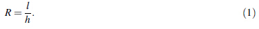

Equation (2) illustrates that the LHRL change causes the time of stacker spending change for the same tasks. Consequently, the warehouse scheduling efficiency is also influenced by it.
 |
| Fig. 2 The structure of rack |
There exists some semi-finished products which have different processes on automation production line, thus they each have different storage time in the warehouse. At the same time, the random of the production is regarded. Therefore, it may cause that those semi-finished products which come out of warehouse at a time compete for the stacker, and then the storage time of the semi-finished products is longer than the normal time to some degree. This problem is even more serious in the case that there are a large number of semi-finished products [15, 16, 17].
In order to quantize the problem, the definitions are as follows.
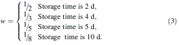
efinition 1 The unit timeout value which affects the degree of the product quality is represented as weight. Depending on the different storage time of product in the warehouse, the weight is defined as follows
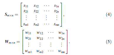
Definition 2 According to the locations of the semifinished products and their storage time in the warehouse, a buffer is opened up in the RAM, in which the storage time matrix Sm × n and the weight matrix Wm × n are generated dynamically corresponding to the semi-finished product in the warehouse, they are defined as
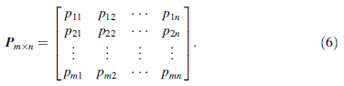
Definition 3 The past time matrix Pm × n nindicates the time pass by the semi-finished products since they have been stored in the warehouse, which is defined as
The scheduling model is described as,

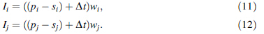
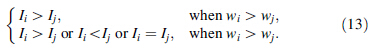
The scheduling will be operated in descending order of Ii, the scheduling sequence is showed as,

As it always takes the stacker a certain amount of time to carry the semi-finished product out of the warehouse, this scheduling sequence (8) shows a local optimum rather than a global optimum, which is proved as follows.
Supposing


As proved above, this scheduling model is time-varying. Therefore, the scheduling sequence needs to be updated dynamically all the time to achieve a global optimum. 4 Utilization of sparse matrix in warehouse scheduling
The matrix Dm × n is defined as the difference between Pm × n and Sm × n, in which the element di indicates the timeout corresponding to the location in the warehouse. That’s to say, it can be represented as


The above method has little effect on the search efficiency when the size of a warehouse is small. Otherwise, it will have a huge influence on the search efficiency. In view of this situation, the rules are defined as follows.
Given a situation that the number of the semi-finished products whose storage time expires is a small part of the whole product in the warehouse in a short period of time, based on which the matrix Dm × n is transformed as follows.
If there are some positions in which there are no semifinished products or the storage time of semi-finished products don’t expire or semi-finished products has been placed the scheduling sequence, the elements of the matrix Dm × n are assigned to zero corresponding to such positions.
The number of zero elements is much larger than the number of non-zero elements by means of such transformation in the matrix Dm × n, so it becomes a sparse matrix, in which only non-zero elements of the matrix are calculated. Then it will improve the calculation and scheduling efficiency greatly. 5 Design of scheduling algorithm based on IoQ strategy
The principle of the scheduling algorithm based on the IoQ parameter is that the IoQs are computed for semi-finished products whose storage time has expired, and the one whose IoQ is the largest scheduled first. With an eye to the different weights and the changing timeout value for such semi-finished products, the IoQs of the rest semi-finished products of the warehouse also keep varying. It is needed to calculate the IoQs to achieve the optimal scheduling on line all the time. The specific scheduling steps are as follows.
Step 1 The mapping two-dimension array a is maintained in RAM according to the size of the warehouse in the actual production. The elements of the table are structure variables which are associated with the semi-finished product. Those variables include the following members:
(i) the warehouse location number of the semi-finished product,
(ii) the storage time of the semi-finished product,
(iii) the weight of the semi-finished product corresponding to the current storage time,
(iv) the start time of the semi-finished product in the warehouse,
(v) the flag which marks whether the semi-finished product has been in the scheduling sequence.
Step 2 The Sm × n, Wm × n and Pm × n are generated from the mapping a at the current time. If the elements of Wm × n are all zero, then goes to Step 1.
Step 3 The Dm × n is worked out by Eq. (14), meanwhile, the matrix Dm × n is transformed to the sparse matrix by the rules of this paper. Then the two-dimension array b is generated whose elements correspond to the non-zero in the sparse matrix Dm × n.
Step 4 The IoQs of the semi-finished products are calculated in b according to Eq. (15) and the maximum value among IoQs is placed on the tail of the scheduling sequence. The flag of the semi-finished product, which identify whether it has been in the scheduling sequence, is set as the number one.
Step 5 Under field conditions, the time which the stacker spends to carry the semi-finished product out of the warehouse passes, then go to Step 1. The following semifinished product in the scheduling sequence is obtained. 6 Experimental verification and analysis
The number of the semi-finished product and their timeout values are assumed in the warehouse, and the following agreement is done.
The perimeter of the location is 3 m. υx and υy are 1 m/s, 0.5 m/s respectively. The products quality or scheduling performance is marked as SoP, which is the sum of the product of the timeout and the weight for every task. The semi-finished products whose timeout value is 10 s is marked as A; in the same way, the semi-finished products whose timeout value is 20 s is marked as B; the semi-finished products whose timeout value is 30 s is marked as C; the semi-finished products whose timeout value is 40 s is marked as D; the semi-finished products whose timeout value is 50 s is marked as E.
The proposed strategy is verified and compared with FCFO [18] strategy and random strategy respectively. On the condition whose platform is Windows XP, frequency is 1.49 GHz, memory size is 1.99 GB, development environment is VC++ 6.0.
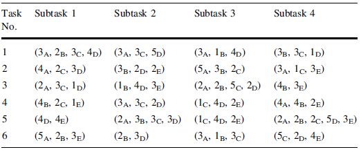
Table 1 shows that the experiments have six tasks, and each task includes four subtasks. And the XY indicates that the number of timeout category which belongs to Y is X. At the same time, the coordinates of six tasks in the warehouse are shown in Fig. 3, of which Xyz means the product belongs to X, the task and the subtask of which are y and z respectively. Besides, different tasks are labeled with different colors. The numbers at the left side and at the top side of Fig. 3 are represented as layer numbers, column numbers respectively.
 |
| Fig. 3 Coordinates of six tasks in the warehouse |
Table 2 states that the IoQ strategy is compared with the other two strategies with six tasks respectively under different LHRLs.
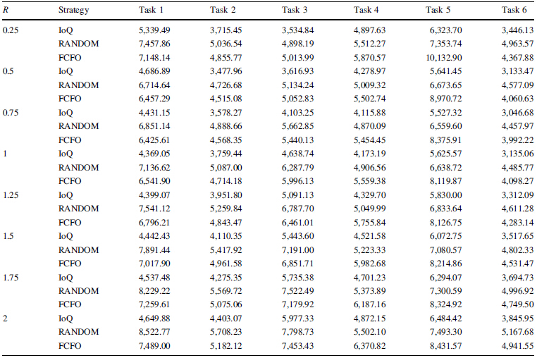 |
From Table 2, it can be seen that the varied LHRL has a great influence on scheduling performance for scheduling strategies. At the same time, the simulation results reveal that the LHRLs corresponding to minimum SoP of different scheduling strategies are different. For example, for the Task 1, the LHRLs corresponding to the minimum SoPs are 1, 0.75 and 0.5 for IoQ, FCFO and RANDOM respectively. Therefore, to get better scheduling performance, it is essential to find a suitable LHRL for different scheduling strategies. Furthermore, it can be observed that the IoQ strategy outperforms the other two scheduling strategies considering all the SoP values, and FCFO is more or less than RANDOM. In other words, the IoQ strategy compared with the others has the smallest impact on the quality of the products.
In order to highlight the advantage of the IoQ relative to the others. The evaluation metric is defined as
 |
| Fig. 4 Product quality improve ratio for IoQ relative to FCFO and random strategies in six tasks |
Figure 4 illustrates that the IoQ strategy improve obviously the scheduling performance compared with the other two strategies under different R. Furthermore, the improvement degree varies as the R changes, and the best improvement ratio even reaches 45.4 % and 37.9 % respectively relative to RANDOM and FCFO. Meanwhile, the LHRL values R are different when themetric Q(a, b) gets the peak value for every tasks, and the reason of which is that the timeout weights are various for every subtasks in every tasks, which implies that there is a suitable R for every task and every scheduling strategy. What’s more, it can be deduced that the IoQstrategy is better than the other two no matter what the R is. Therefore, it is also proved that the proposed IoQ strategy is more effective for improving scheduling performance considering the changes of R. In a word, this paper provides a sound theoretical base for the design of the automated warehouse. 7 Conclusions
This paper investigated how the LHRL affects the scheduling performance. Meanwhile, the IoQ mathematical model is built, which is based on the idea that the extent of the unit timeout value which has influence on the product quality. Besides, the scheduling strategy with IoQ is designed. The experiment is performed by scheduling the semi-finished products with different storage time in the warehouse. Comparing with warehouse scheduling strategies, the results show that R has different effect on scheduling performance for different scheduling strategies, and there is a proper R for the best scheduling performance of each scheduling strategy. Additionally, the proposed strategy greatly improves the scheduling performance compared with the other two R changing conditions.
Acknowledgments This work is supported by the National Natural Science Foundation of China (Grant Nos. 61074032 and 61273040), the Project of Science and Technology Commission of Shanghai Municipality (Grant No. 10JC1405000), and the Shanghai Rising-Star Program (Grant No. 12QA1401100).| 1. | Hachemi K, Sari Z, Ghouali N (2012) A step-by-step dual cycle sequencing method for unit-load automated storage and retrieval systems. Comput Ind Eng 63(4):980-984 |
| 2. | Ekren BY, Heragu SS, Krishnamurthy A et al (2013) An approximate solution for semi-open queueing network model of an autonomous vehicle storage and retrieval system. IEEE Trans Autom Sci Eng 10(1):205-215 |
| 3. | Gagliardi JP, Renaud J, Ruiz A (2012) Models for automated storage and retrieval systems: a literature review. Int J Prod Res 50(24):7110-7125 |
| 4. | Hu G, Kise H, Xu Y (2005) Optimization for input/output scheduling for automated warehouses. Trans Inst Syst Control Inf Eng 18(4):156-163 |
| 5. | Chan FTS, Kumar V (2009) Hybrid TSSA algorithm-based approach to solve warehouse-scheduling problems. Int J Prod Res 47(4):919-940 |
| 6. | de Reneé K, Tho LD, Kees JR (2007) Design and control of warehouse order picking: a literature review. Eur J Oper Res 182(2):481-501 |
| 7. | Basile F, Chiacchio P, Coppola J (2012) A hybrid model of complex automated warehouse systems-part i: modeling and simulation. IEEE Trans Autom Sci Eng 9(4):640-653 |
| 8. | Estanjini RM, Lin YW, Li KY et al (2011) Optimizing warehouse forklift dispatching using a sensor network and stochastic learning. IEEE Trans Ind Inf 7(3):476-486 |
| 9. | Luo J, Wu CQ, Li B et al (2011) Modeling and optimization of RGV system based on improved QPSO. Comput Integr Manuf Syst 17(2):321-328 |
| 10. | Yu MF, Koster RD (2010) Enhancing performance in order picking processes by dynamic storage systems. Int J Prod Res 48:4785-4806 |
| 11. | Liu CQ, Li MJ, Chen XB (2009) Order picking problem based on ant colony algorithm. Syst Eng Theory Pract 29(3):179-185 |
| 12. | Li MJ, Chen XB, Zhang MF (2007) Path planning based on the swarm intelligence algorithm. J Tsinghua Univ (Sci & Tech) 47(z2):1770-1773 |
| 13. | Chen L, Langevin A, Riopel D (2011) Dynamic relocation problem in an automated storage/retrieval system. J Shanghai Jiaotong Univ 45(1):115-119 |
| 14. | Lerher T, Sraml M, Potrc I et al (2010) Travel time models for double-deep automated storage and retrieval systems. Int J Prod Res 48(11):3151-3172 |
| 15. | Chang FL, Liu ZX, Xin Z et al (2007) Research on order picking optimization problem of automated warehouse. Syst Eng Theory Pract 2:139-143 |
| 16. | Shi N (2010) K constrained shortest path problem. IEEE Trans Autom Sci Eng 7(1):15-23 |
| 17. | Liu SN, Ke YL, Li JX et al (2006) Optimization for automated warehouse based on scheduling policy. Comput Integr Manuf Syst 12(9):1438-1443 |
| 18. | Vandevelde G, Gademann N, Vandevelde S (2005) Order batching to minimize total travel time in a parallel-aisle warehouse. IIE Trans 37(1):63-75 |