 2016, Vol. 4
The article information
- Guo Shuai, Jin Yi, Bao Sheng, Xi Feng-Feng
- Accuracy analysis of omnidirectional mobile manipulator with mecanum wheels
- Advances in Manufacturing, 2016, 4(4): 363-370.
- http://dx.doi.org/10.1007/s40436-016-0164-3
-
Article history
- Received: 10 January, 2016
- Accepted: 11 November, 2016
- Published online: 9 October, 2016


2 Department of Aerospace Engineering, Ryerson University, Toronto, Canada
Recently, with the development of industrial robots, the mobile robots have been used in various industries. Compared to traditional mobile robots, the omnidirectional mobile robots have a broad application prospect in aerospace and other fields, as it can move in any direction and its turning radius can be zero. Mecanum omnidirectional mobile platform is a popular omnidirectional mobile robot. It can flexibly complete various tasks in crowded space.
The mobile platform built for riveting the rocket skin is shown in Fig. 1, which includes a mecanum omnidirectional mobile platform, laser sensors, a manipulator with six degrees of freedom. In order to make the mobile platform move precisely, we need to revise its movement equation. Muir and Neuman [1] have developed a kinematic model of mecanum robot using matrix theory. Wang and Chang [2] carried out error analysis interns of distribution with four mecanum wheels. Shimada et al. [3] introduced a position corrective feedback control method using a vision sensor on mecanum-wheel omnidirectional vehicles. Qian et al. [4] developed a more detailed analysis on the installation angle of roller. This paper does a further study from the perspective of the deformation of the roller and provides two methods to revise its movement equation.

|
| Fig. 1 3D-model of the mobile robot |
Figure 2 shows the prototype robotic system built at Shanghai University. According to kinematic analysis [5], its motion equation is shown as

|
| Fig. 2 a Prototype robotic system, b motion model |
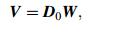
where 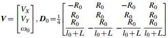

Figure 3 is a view of a mecanum wheel and a roller. The roller is fitted on the edge of the mecanum wheel in angle a with its central axis, which can rotate freely around its central axis. The wheel relies on the friction that the roller acts on the ground to move. Because the material of its outer rim is usually rubbers, it will deform under pressure.

|
| Fig. 3 Mecanum wheel and roller |
Figure 4 is a view of distribution of roller outer rim deformation in its transverse section. F is the pressure on the roller, T the driving torque. The radiuses of wheels reduce differently under different pressures. The greater the pressure, the greater the deformation is. The deformation zone shifts with the action of driving torque and the shifting causes the position of wheel center to change. From the force analysis of mecanum wheel [6], we know that with the wheel rotating, a driving torque is generated by the force in roller axial direction, so the position of the contact points will shift in axial direction. With the deformation of the roller, the R0 and l0 will change.

|
| Fig. 4 Distribution of roller deformation |
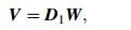
Based on the kinematic analysis of omnidirectional mobile system and deformation of the roller [7-16], Eq. (1) can be revised to individual parameters.
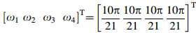
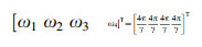
The model is established in Fig. 5, a coordinate system XOY is set at the center O of the model; VX, VY, ω0 are defined as the linear and angular speeds of platform movement, respectively. ω1, ω2, ω3 and ω4 are angular velocities of the wheels; l1, l2, l3 and l4 are the distances from the wheel centers O1, O2, O3 and O4 to the platform center O in X-direction; R1, R2, R3 and R4 are the radiuses of four wheels, respectively. The direction of the arrow indicates the positive direction.

|
| Fig. 5 Motion model of mobile platform |
In order to improve the system motion accuracy, we should solve the relative errors ΔRi between Ri and R0, and relative errors Δli between li and l0 (i=1, 2, 3, 4) to revise matrix D1 in Eq. (2).
3 Method of solution 3.1 Relative error matrixAfter multiplying time t, Eq. (2) becomes displacement equation

where 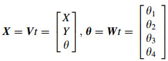
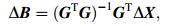
Then the relative errors can be determined by
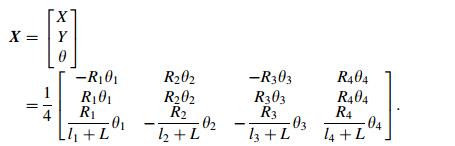
Differentiating Eq. (4) leads to

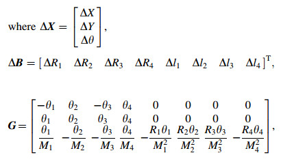
Then the relative errors can be determined as
among them, Mi=li + L cosα, θi=ωit (i=1, 2, 3, 4).
In order to carry out simulation, we need to verify whether the above method is feasible. From manufacturing and assembly tolerances to define ΔRi the deformation of the roller and Δli in [-h, h] and [-j, j] (h=3; j=5).
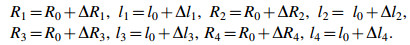
The li and Ri can be written as
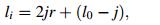
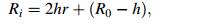
where li and Ri are in [lo-j, lo + j] and [Ro-h, Ro + h], respectively; r is a random number between 0 and 1.
Define ω1=ω2=ω3=ω4=20 rad; t=1 s. The rank of matrix G is 3. G is a full rank matrix. So ΔB satisfies Eq. (6).
3.2 Solution of relative errors 3.2.1 Displacement error measurementIn order to obtain matrix ΔB, we need to obtain displacement error matrix ΔX firstly. Assuming that the deformation of the rollers exists and the ground condition is good, four wheels of the platform can touch the ground [17].
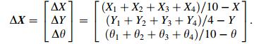
Set matrix 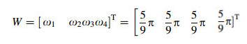
The principle of measurement is shown in Fig. 6 and matrix ΔX can be obtained as

|
| Fig. 6 The principle of measuring displacement |
According to Eq. (1), X, Y and θ can be obtained as X=VXt=0, Y=VYt=2R0ω1=654 mm, θ=2ω0=0.
Finally, through the experiment we obtain the displacement errors
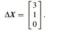 (10)
(10) Take Eq. (10) to Eq. (6) and use interval analysis and Monte Carlo analysis to obtain matrix ΔB:
3.2.1.1 Monte Carlo analysisThis method comes from Monte Carlo method. In Eqs. (7) and (8), li and Ri are the assigned random values. Take them into matrix G and Eq. (6) to obtain matrix ΔB.
As the value of ΔX has been obtained in Eq. (10), take the random values of li and Ri into Eq. (6), we can obtain the corresponding matrix ΔB which also needs to satisfy that -3≤ΔRi≤3 and -5≤Dli≤5, solve matrix ΔB N times (N → ∞) until obtain 50 groups of matrix ΔB. It also means that through the displacement error ΔX in Eq. (10), we find 50 groups of matrix ΔB and its corresponding random matrix G.
We also obtain 50 groups of ΔR1; ΔR2; ΔR3; ΔR4; ΔR1; ΔR2; ΔR3; ΔR4 (see Fig. 7).

|
| Fig. 7 The values obtained in Monte Carlo method |
Average the 50 groups of ΔR1; ΔR2; ΔR3; ΔR4; ΔR1; ΔR2; ΔR3; ΔR4 to form a new matrix ΔB1=[-0.541 1.237-0.605 1.055 0.458 0.683-0.048-0.683]T. Now we use process capability index to estimate the value of matrix ΔB1. Process capability, also known as working procedure capability, refers to the ability that process machining meets the machining quality. It is a measure of the minimum fluctuation of the internal consistency of process machining in the stablest state. When the process is stable, the quality characteristic value of product is in [μ-3σ, μ + 3σ] (μ is ensemble average of quality characteristic value of product, σ standard deviation of quality characteristic value of product), so this can be used to estimate the stability and accuracy of quality characteristic value of product.
There are two kinds of situations to solve process capability index. Firstly, μ=M is shown in Fig. 8. USL is the maximum machining error of machining quality; LSL is the minimum machining error of machining quality; M=(USL + LSL)/2; μ is the average value of process machining. Cp indicates process capability index, Cp=(USL -LSL)/6σ.

|
| Fig. 8 μ=M |
Secondly, μ ≠ M is shown in Fig. 9.

|
| Fig. 9 μ ≠ M |
Cpk indicates process capability index, Cpk=(USL -LSL)/6σ -|M -μ|/3σ.
Only process capability index is greater than 1, and the value of process machining is valid.
As -3≤ΔRi≤3 and -5≤Δli≤5, M=0 and μ ≠ M, we can obtain: Cpk(ΔR1)=1.58>1, Cpk(Δl1)=0.57<1, Cpk(ΔR2)=1.06>1, Cpk(Δl2)=0.58<1, Cpk (ΔR3)=1.54>1, Cpk(Δl3)=0.63<1, Cpk(ΔR4)=1.17>1, Cpk(Δl4)=0.5<1.
So the values of ΔR1, ΔR2, ΔR3 and ΔR4 in ΔB1 are closer to the real values than the values of ΔR1, ΔR2, ΔR3 and ΔR4 in ΔB.
Now take matrix ΔB1(a)=[-0.541 1.237-0.605 1:055 0 0 0 0]T; ΔB1(b)=[0 0 0 0 0.458 0.683-0.048-0.683]T into Eq. (5), we obtain ΔX1(a)=[-0.4119 4-0.003]T, ΔX1(b)=[0 0 0.0032]T.
According to the change rate of them relative to Eq. (10), the influence of ΔR1, ΔR2, ΔR3 and ΔR4 is much bigger than that of Δl1, Δl2, Δl3 and Δl4. Although the values of Δl1, Δl2, Δl3 and Δl4 are not accurate enough for the real values, matrix DB1 is valid.
3.2.1.2 Interval analysisIn Eq. (6), matrix G is uncertain because of the change of ΔRi and Δli in [-3, 3] and [-5, 5], respectively. Now we set the increment of ΔRi and Δli is 1 mm, there are 7 values of ΔRi, and 11 values of Δli, so there are 74 × 114 groups of combination of matrix G. Take all the combination of matrix G to Eq. (6) to obtain matrix ΔB and exclude the combination of matrix ΔB that ΔRi and Δli are not in [-3, 3] and [-5, 5], respectively. So we obtain 277 groups of matrix ΔB.
Average the values in Fig. 10 and obtain the average values of ΔR1; ΔR2; ΔR3; ΔR4; Δl1; Δl2; Δl3; Δl4. Use the average values to combine a new matrix ΔB2=[-0.233 1.467-0.923 0.824 0.2-0.213 -0.068 -0.039]T.

|
| Fig. 10 The values obtained in interval analysis |
Use the same way to solve the process capability index of ΔB2, we can obtain: Cpk(ΔR1)=3.34>1, Cpk (Δl1)=0.68<1, Cpk(ΔR2)=1.22>1, Cpk(Δl2)=0.59<1, Cpk(ΔR3)=2.5>1, Cpk(Δl3)=0.63<1, C pk (ΔR4)=1.73>1, Cpk(Δl4)=0.6<1.
So the values of ΔR1, ΔR2, ΔR3 and ΔR4 in ΔB2 are closer to the real ones than the values of Δl1, Δl2, Δl3 and Δl4 in ΔB2. As the influence of ΔR1, ΔR2, ΔR3 and ΔR4 is much bigger than Δl1, Δl2, Δl3 and Δl4, matrix ΔB2 is valid.
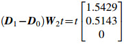
3.2.2 Result validationUse the matrix ΔB1 to revise the parameters of matrix D1 in Eq. (2), we obtain 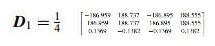

Use the same way to calculate with matrix ΔB2, we can achieve 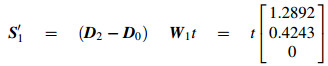
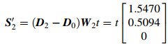
Set t=2 to measure the displacement errors, compare the values of measuring with S1 and S2.
Figure 11(a) is the entire experiment with 4 movements. Figure 11(b) is the image of actual movement. From the comparison, we find that S1, S2 are close to the measured displacement errors, so ΔB1 and ΔB2 are satisfied to revise the matrix D1.

|
| Fig. 11 Schematic diagram of measuring and the actual measuring |
Through analyzing the roller deformation of mecanum wheel, we can find the changed parameters of the motion equation of mobile system. In this paper, the relative variation of the parameters in the motion equation of the mecanum motion platform is solved by Monte Carlo analysis and interval analysis. Using the relative variation of the parameters to revise the motion equation, then solve the displacement errors in different spaces in theory and compare them with the measured displacement errors in fact. From the comparison, both the two methods are satisfied to requirement.
Acknowledgements This work was supported by the Shanghai Municipal Science and Technology Commission (Grant Nos. 14111104502 and 15550721900).| 1. | Muir PF, Neuman CP (1987) Kinematic modeling for feedback control of an omnidirectional wheeled mobile robot. In:Proceedings of the 1987 IEEE international conference on robotics and automation, pp. 1772-1778 |
| 2. | Wang Y, Chang D(2009) Preferably of characteristics and layout structure of mecanum comprehensive system. J Mech Eng, 45(5), 307-310 doi:10.3901/JME.2009.05.307 |
| 3. | Shimada A, Yajima S, Viboonchaicheep P et al (2005) Mecanumwheel vehicle systems based on position corrective control. In:proceedings of the 2005 IEEE annual conference on industrial electronics society |
| 4. | Qian J, Wang X, Xia G(2010) Velocity rectification for mecanum wheeled omni-direction robot. Manuf Technol Mach Tools(11), 42-45 |
| 5. | Zhou L, Wu H(2011) Machine design and manufacturing engineering. Int J Mach Tools Manuf, 40(5), 2193-2211 |
| 6. | Zhang P (2011) Kinematics simulation analysis and structural topology optimization of omni-directional mobile transport platform. Dissertation, Nanjing University of Aeronautics and Astronautics |
| 7. | Chen X, Kong L, Liu Z(2012) Motion analysis and control design of moving mechanism of robot based on omni-directional wheel. Meas Control Technol, 31(1), 48-51 |
| 8. | Huang D, Jia Q, Zhu Q, et al(2015) Motion analysis and structure design of mecanum wheeled robot. Sci Technol Innov Herald, 2015(19), 4-5 |
| 9. | Bottema O, Roth B(1990) Theoretical kinematics. Dover Publications, New York, pp, 165 |
| 10. | Indiveri G(2009) Swedish wheeled omnidirectional mobile robots:kinematics analysis and control. IEEE Trans Robot, 25(1), 164-171 doi:10.1109/TRO.2008.2010360 |
| 11. | Salih J, Rizon M, Yaacob S, et al(2006) Designing omni-directional mobile robot with mecanum wheel. Am J Appl Sci, 3(5), 1831-1835 doi:10.3844/ajassp.2006.1831.1835 |
| 12. | Li L, Ye T, Tan M, et al(2003) Current situation and future of mobile robot technology. Robot, 24(5), 475-480 |
| 13. | Xu G, Tan M(2001) Development status and trends of the mobile robot. Robot Technol Appl, 3, 1-3 |
| 14. | Zhao D(2010) Easy to build and strong. Introduction omnidirectional mobile robot. Beijing, pp , Science Press , 3 -5 |
| 15. | Chang Yi(2007) Mobile robotics and its application. , Electronic Industry Press , 11 -12 |
| 16. | Martinelli A, Tomatis N, Siegwart R(2007) Simultaneous localization and odometry self calibration for mobile robot. Autonomous Robots, 22(1), 75-85 |
| 17. | Jung C, Chung W(2011) Calibration of kinematic parameters for two wheel differential mobile robots by using experimental heading errors. Int J Adv Robot Syst, 8(5), 134-142 |
| 18. | Wang B, Ma C, Wen B(2013) Design of omni-driection mobile platform based on three mecanum wheels. J Mech Electr Eng, 30(11), 1358-1362 |
| 19. | Liu Z, Zhang C, Wang Z(2013) Omnidirectional mobile platform motion analysis and simulation. Mach Electron, 2013(8), 16-19 |
| 20. | Wang X(2014) Introduction of mecanum-wheels based omnidirectional mobile robots with applications. Mach Build Autom, 43(3), 1-6 |
| 21. | Jia G (2012) Research on theory and application of an omnidirectional platform with mecanum wheel. Zhejiang University, Zhejiang |