在遥感观测数据中，由于地物光谱特征的多样性和传感器空间分辨率的限制，导致观测结果中普遍存在混合像元(Hui 等，2007)。而混合像元的存在是遥感向定量化深入研究的重要障碍(Lv 等，2003)，为解决该问题，国内外研究提出了多种混合像元分解模型，主要包括线性光谱混合模型LSMM(Linear Spectral Mixture Model)、概率模型(Probabilistic Model)、几何光学模型(Geometric-optical Model)、随机几何模型(Stochastic Geometric Model)和模糊模型(Fuzzy Model)等(Charles和Karnieli，1996)。在以上光谱混合模型中，线性光谱混合模型因其在理论上有较好的科学性，物理意义简单明确，得到了广泛的应用(Chen 等，2016)。

由于地球表面的复杂性和遥感观测多时空分辨率的特点，使得遥感影像获取的地面信息具有很大的跨度(Li 等，2000, 2002)，所以从遥感出发的地学描述必然存在多尺度问题(Li和Wang，2013)。而在实际应用中，往往需要根据不同的情况选择合适的尺度(Curts 等，1987)，因此，在描述不同的地学现象和地表过程时，必须考虑尺度效应的影响(Luan 等，2013；Chen，1999)。遥感尺度主要是空间的尺度，包括空间分辨率和空间范围，空间尺度效应的研究通常分为以下两个方面：一方面是在特定尺度下研究遥感物理定律、定理、模型以及概念的修正，另一方面，则是针对不同观测尺度或者空间分辨率下获取的参数之间的变异以及变化规律进行分析(Huang 等，2016；Wan 等，2008)。

线性光谱混合模型虽然是解决宏观观测尺度下混合像元分解的简单、有效的方法，在微观观测尺度时却不再适用(Li，2004；Liu和Li，2014)。为进一步探究线性光谱混合模型的解混效果随观测尺度改变的变化规律，本文由地物辐射原理出发，首先推导了微面元辐射通量和积分线性光谱混合模型的表达式，然后在假定地物取均一反射率和数值模拟随机反射率两种情况下，分别计算了两模型的相对差值Δρ，结合室外和室内实验实测光谱数据验证，从而证明了半瞬时视场角(β)的大小可作为确定线性光谱混合模型适用观测尺度的关键依据。

在混合像元中，地物端元可视为由众多相同反射率的微面元组成，某一波长处的混合光谱应为该波长处所有微面元有效辐射能量的总和。首先从地物辐射特性出发，推导地物微面元在探头处辐射通量的表达式，并在此基础上建立积分线性光谱混合模型ILSMM(Integral Linear Spectrum Mixture Model)。

以非成像光谱仪测量为例，当光谱仪探头垂直于水平地表观测时，设观测高度为H，光谱仪探头半瞬时视场角s-IFOV(semi-Instantaneous Field of View)为β，探头的中心点为A，面积为dA，点A在被测地物表面的投影为O，观测范围为以O点为圆心，R为半径的圆，可得

$R = H\tan \beta $

(1)

假设光谱仪视域中某一地物端元为朗伯体，辐射亮度为L，其上存在一个微面元，中心点为B，面积为dS，AO与AB的夹角(即天顶角)为θ(图1)。

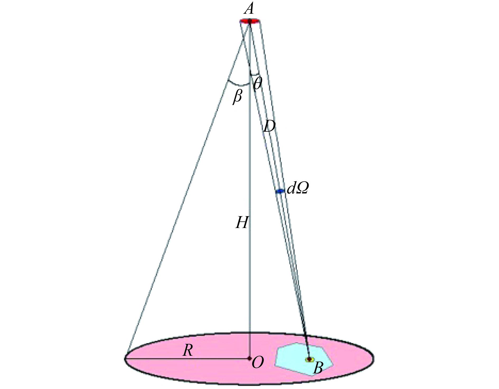
由式(1)可得A、B两点间距离D为

$D = \frac{H}{{\cos \theta }}$

(2)

点B在光谱仪探头方向所成的立体角为(赵英时 等，2013)

$d\varOmega = \frac{{dA\cos \theta }}{{{D^2}}} = \frac{{dA{{\cos }^3}\theta }}{{{H^2}}}$

(3)

设在某一固定波长处，微面元在光谱仪探头入瞳处的有效辐射通量为dM，根据辐射亮度的定义(Zhao，2013)，可得

$dM = L \cdot d\varOmega \cdot dS\cos \theta $

(4)

将式(3)代入式(4)得

$dM = L \cdot dS \cdot \frac{{dA{{\cos }^4}\theta }}{{{H^2}}}$

(5)

由朗伯体辐射特性可知，在半球空间内，该朗伯体地物的辐射出射度为πL(Zhao，2013)，设地物表面垂直入射的辐照度为E，地物反射率为ρ，则应有

$\rho E = {\text{π}} L$

(6)

将式(6)代入式(5)得：

$dM = \frac{{\rho E}}{{\text{π}}} \cdot dS \cdot \frac{{dA{{\cos }^4}\theta }}{{{H^2}}}$

(7)

结合式(1)和式(7)，可得

$dM = \rho E \cdot dS' \cdot dA{\cos ^4}\theta {\tan ^2}\beta $

(8)

式中，dS′代表该微面元的面积比。

微面元B具有任意性，因此，由该式可知，dM除了受到端元反射率和面积比的影响外，也与天顶角存在非线性关系，θ越大，对dM的影响越显著。为进一步分析微面元辐射通量与混合光谱之间的关系，在微面元辐射通量的基础上推导了积分线性光谱混合模型的表达式。

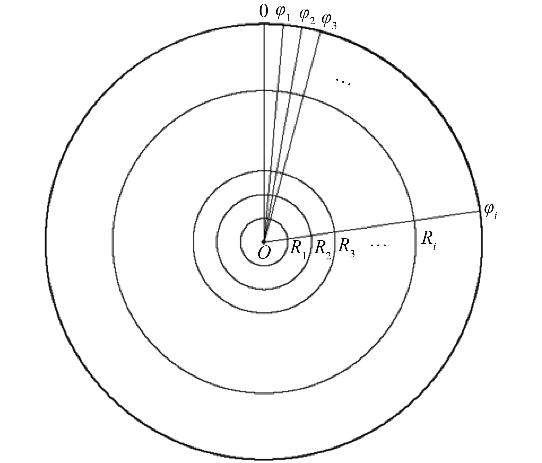
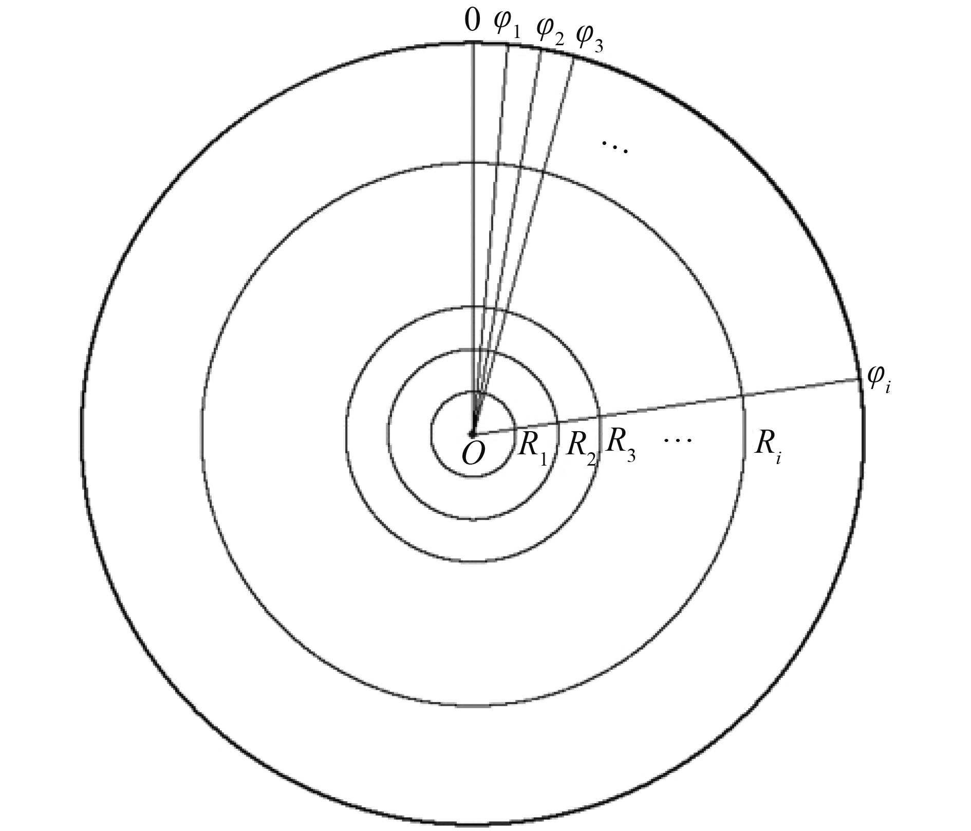
混合光谱应是观测视域内所有地物微面元有效辐射能量的线性组合，为推导ILSMM的表达式，采用以下方法将观测范围划分为微面元：首先，以O为圆心，R_i为半径作圆，其中，0<R₁<R₂< $ \cdots $ <R_i< $ \cdots $ R_n−1<R(R_i+1−R_i=dr, n→∞)；再以O为顶点，取0<φ₁<φ₂< $ \cdots $ <φ_i< $ \cdots $ φ_m−1<2π(φ_i+1−φ_i=dφ, m→∞)，将方位角在2π范围内进行m等分(图2)。这样将观测视域内的地物端元分割为很多扇弧形微面元，设微面元的总个数为N。

首先假定观测地物为单一朗伯体，则该地物在各方向上的辐射亮度和各处反射率都相等。设在某一波长处，微面元的辐射亮度为L_K，反射率为ρ_K，因为反射率连续且相等，根据式(7)，地物的总辐射通量M_K可由下式计算

${M_K} = \iint {\frac{{{\rho _K}E}}{{\text{π}}}} \cdot dS \cdot \frac{{dA{{\cos }^4}\theta }}{{{H^2}}}$

(9)

式中，扇弧形微面元面积为(图3)

$dS = \frac{1}{2}d\varphi \left( {{{\left({r + dr} \right)}^2} - {r^2}} \right) = rdrd\varphi + \frac{1}{2}d\varphi d{r^2}$

(10)

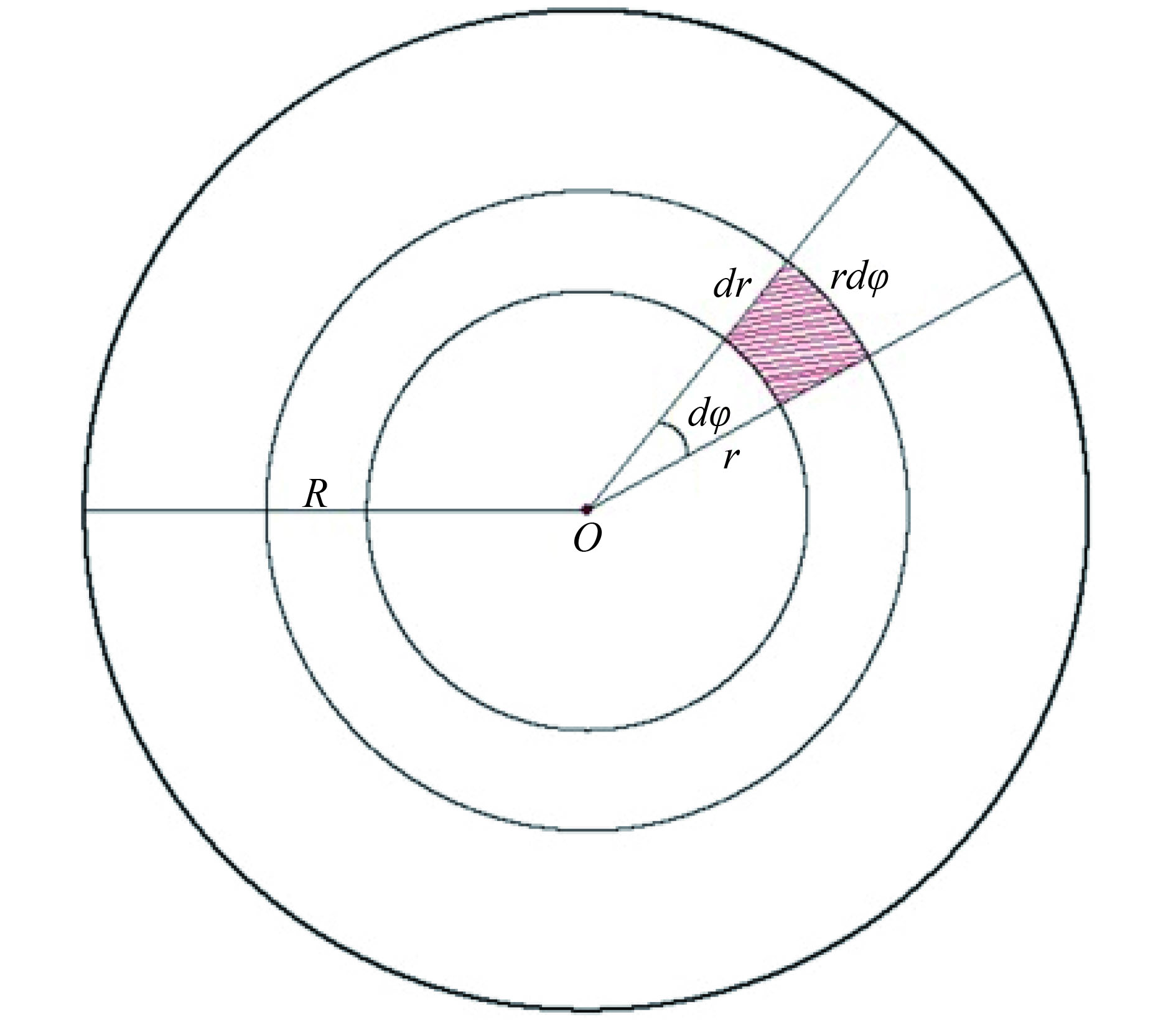
因为dr、dφ均为微小值，可忽略不计，因此微面元的面积可以近似为

$dS = rdrd\varphi $

(11)

又因为r=Htanθ，可得

$dr = \frac{H}{{{{\cos }^2}\theta }}d\theta $

(12)

把式(11)和式(12)代入式(9)，得到M_K的表达式

${M_K} = \frac{{{\rho _K}E}}{{\text{π}}} \cdot dA\mathop \int \limits_0^{2{\text{π}}} d\varphi \mathop \smallint \limits_0^\beta \sin \theta \cos \theta d\theta $

(13)

化简整理得

${M_K} = {\rho _K}E \cdot \sin{^2}\beta \cdot dA$

(14)

光谱仪探头对其观测范围所成立体角为

$\varOmega = 2{\text{π}} \left({1 - \cos \beta } \right)$

(15)

设混合地物反射率为ρ_T，结合式(4)和式(15)，光谱仪测得的地物总辐射通量M_T应为

${M_T} = \frac{{{\rho _T}E}}{{\text{π}} } \cdot 2{\text{π}} \left({1 - \cos \beta } \right) \cdot dA$

(16)

根据能量守恒，由式(14)和式(16)可得出

${\rho _T} = \frac{{{\rho _K}{{\sin }^2}\beta }}{{2\left({1 - \cos \beta } \right)}}$

(17)

即在观测地物为单一朗伯体情况下，地物反射率为ρ_K时，理论上测得的地物反射率应为ρ_T。

而在LSMM中，认为某一光谱波段中像元的反射率为其端元组分的特征反射率和各自面积比例作为权重系数的线性组合(Li，2008)。因此，若按照LSMM，在该条件下混合光谱理论测量结果应为

${\rho _S} = \mathop \sum \limits_{i = 1}^N \frac{{{\rho _K}d{S_i}}}{{{\text{π}} {R^2}}} = {\rho _K}\mathop \sum \limits_{i = 1}^N \frac{{d{S_i}}}{{\pi {R^2}}}$

(18)

显然，式(18)计算结果为ρ_K。

式(17)建立在观测地物为单一朗伯体的特定条件下。为推导ILSMM在任意情况下的表达式，假设观测范围内的地物均为朗伯体，各微面元的反射率取随机值，在某一波长处，第i个微面元的反射率为ρ_i，对应的天顶角为θ_i，面积为dS_i。由式(8)可知，在光谱仪视域范围内的N个微面元的辐射通量总和应为

${M_N} = \mathop \sum \limits_{i = 1}^N {\rho _i}E \cdot dS_i' \cdot dA{\cos ^4}{\theta _i}{\tan ^2}\beta $

(19)

由式(16)和式(19)，得出ILSMM的表达通式

${\rho _T} = \frac{{{{\tan }^2}\beta }}{{2\left({1 - \cos \beta } \right)}}\mathop \sum \limits_{i = 1}^N {\rho _i}dS_i'{\cos ^4}{\theta _i}$

(20)

若按照LSMM，在上述条件下，混合像元反射率应为

${\rho _S} = \mathop \sum \limits_{i = 1}^N {\rho _i}dS_i'$

(21)

通过以上两种情况的讨论，发现ILSMM与LSMM有一定的相似性，两模型都考虑了端元反射率和面积比对混合光谱的作用，但是LSMM未考虑天顶角的影响。

为分析在不同观测尺度下天顶角对混合光谱的影响和两模型的关系，以ILSMM为基准，按照下式计算两种模型的相对差值

$\Delta \rho = \frac{{{\rho _S} - {\rho _T}}}{{{\rho _T}}}$

(22)

首先，当观测范围内地物为朗伯体并且反射率均一时，根据式(17)和式(22)，整理可得

$\Delta \rho = {\tan ^2}\left({\frac{\beta }{2}} \right)$

(23)

所以，在上述条件下， $\Delta \rho = {\tan ^2}\left({\displaystyle\frac{\beta }{2}} \right)$ ，两者为确定性关系。

β越小，光谱仪观测高度与视域半径的比值越大，代表观测尺度越大，因此可通过改变β的值来得到不同的观测尺度。由于在实际观测中存在多种地物，为在普适性情况下研究两者的关系，假定在观测范围内，各微面元的面积、反射率均取随机值，考虑到实际情况难以满足该条件，采用数值模拟的方法来进一步讨论两者关系。

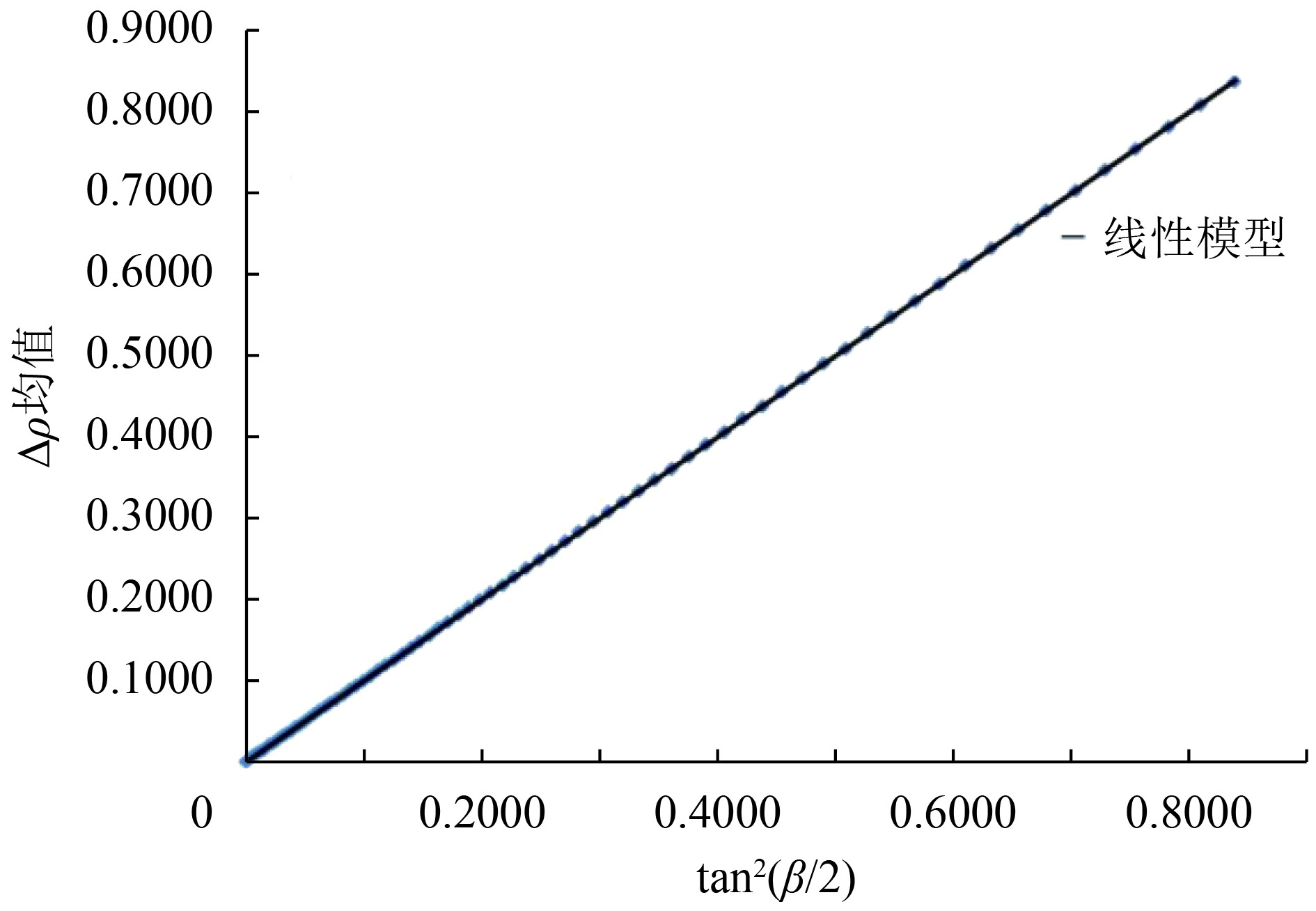
计算机数值模拟过程如下：设β的取值范围为[1, 85]，单位为度，步长为1。按照图2划分观测范围，取n=100，m=360，将观测视域分为N=36000个扇弧形微面元，所有微面元反射率同时在(0，1)取随机值。所有微面元取随机值后，按式(22)在各β处计算Δρ，共模拟5000组反射率，最后求取在各β处的5000组Δρ的均值( $\bar \Delta \rho $ )和标准差(S_Δρ)。

采用SPSS18.0中的线性回归模型y=Kx对 $\bar \Delta \rho $ 和 ${\tan ^2}\left({\displaystyle\frac{\beta }{2}} \right)$ 进行回归分析(图4)，两变量的线性相关系数R²=1，回归方程为

$\bar \Delta \rho = 0.9993\,\,{\tan ^2}\left({\frac{\beta }{2}} \right)$

(24)

在给定信度α=0.05下，对回归方程进行F检验，F=1.746×10⁸，临界值F_α(1，80)=3.96，F>F_α，说明该回归方程有效。

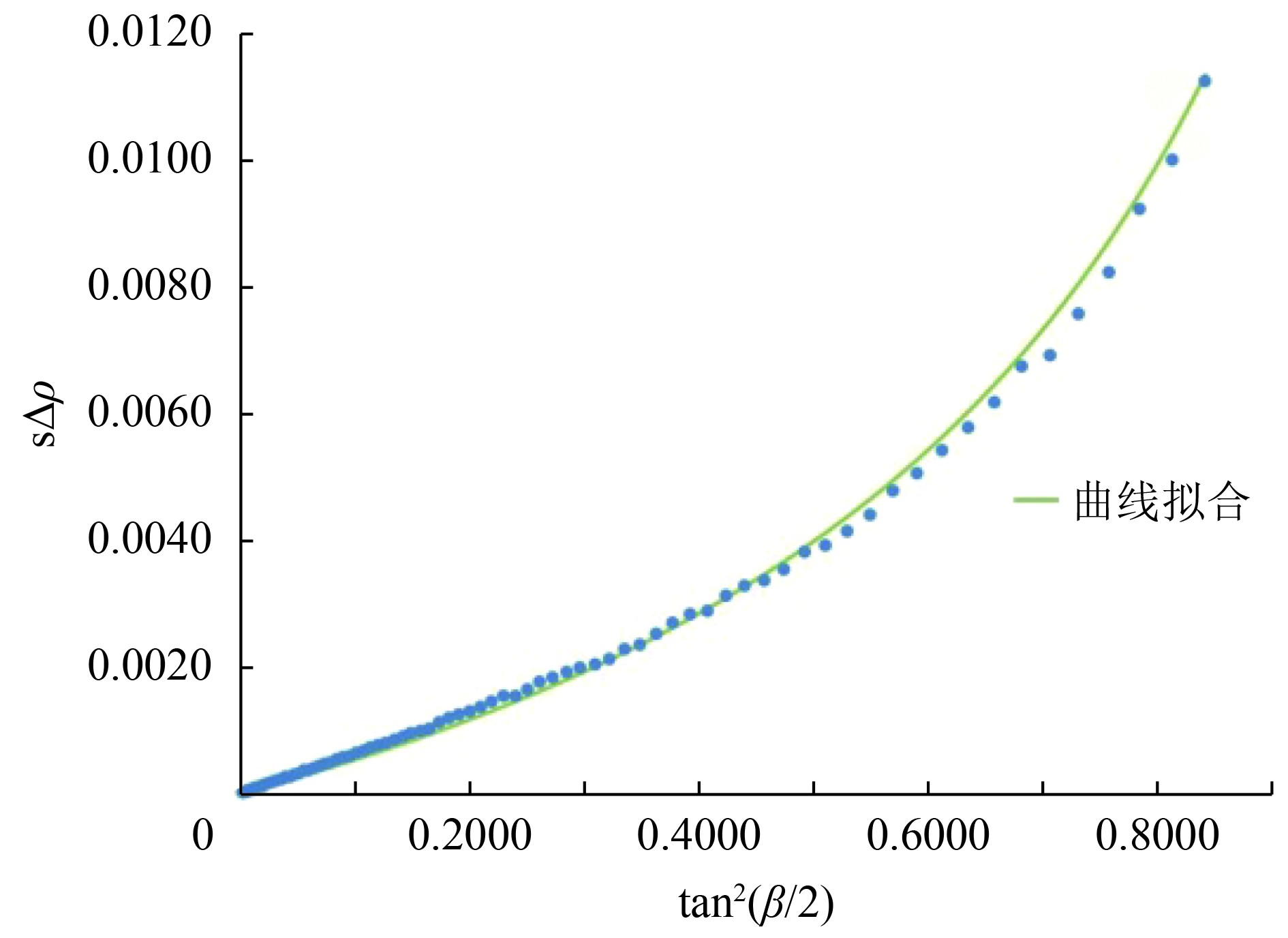
由于直接推导S_Δρ的表达式极为繁琐，因此采用曲线拟合的方式分析β与S_Δρ的关系。对 ${\tan ^2}\left({\displaystyle\frac{\beta }{2}} \right)$ 和S_Δρ进行回归分析(图5)，两者相关系数R²=0.9988，拟合表达式如下

${S_{\Delta \rho }} = 0.0050/\left( {1/\tan{^2}\left({\frac{\beta }{2}} \right) - 0.7500} \right)$

(25)

对各β处的5000组Δρ进行统计分析，绘制概率密度函数分布曲线并计算各曲线的峰度和偏度。与正态分布的峰度(b_k)=3，偏度(s_k)=0相比，所有分布曲线的峰度值均大于3，且3<b_k<5；偏度值为41正，44负，0<|s_k|<0.2，因此Δρ呈现有偏尖峰分布。为进一步了解Δρ的分布特征，根据下式计算各β处Δρ的标准差系数V(周冶芳，2001)

$V = \frac{{{S_{\Delta \rho }}}}{{\bar \Delta \rho }}$

(26)

得到V的取值范围为[0.60%，1.34%]，表明Δρ分布的离散程度很小， ${\bar \Delta \rho }$ 的代表性很高并且数据的稳定性较好。

已有数据表明(赵英时等，2013)，航空成像光谱仪的IFOV一般为1.0—3.0 mrad，少数小于1 mrad；航天成像光谱仪可分为中分辨率和高分辨率两种，在观测高度为705 km时，MODIS的最大IFOV约为1.4 mrad，Hyperion的IFOV约为0.04 mrad，以上成像光谱仪的观测高度均远远大于观测视域半径，因此，航空或航天成像光谱仪获取的遥感图像可视为在宏观尺度下的观测结果。由上述内容可知，在进行宏观尺度观测时，两模型的Δρ较小，此时选用LSMM进行混合像元分解也可以得到理想的结果。但随着观测尺度的降低，天顶角的作用不能忽略，两模型的差异逐渐增大，LSMM不再适用，需按照ILSMM进行混合像元的分解。

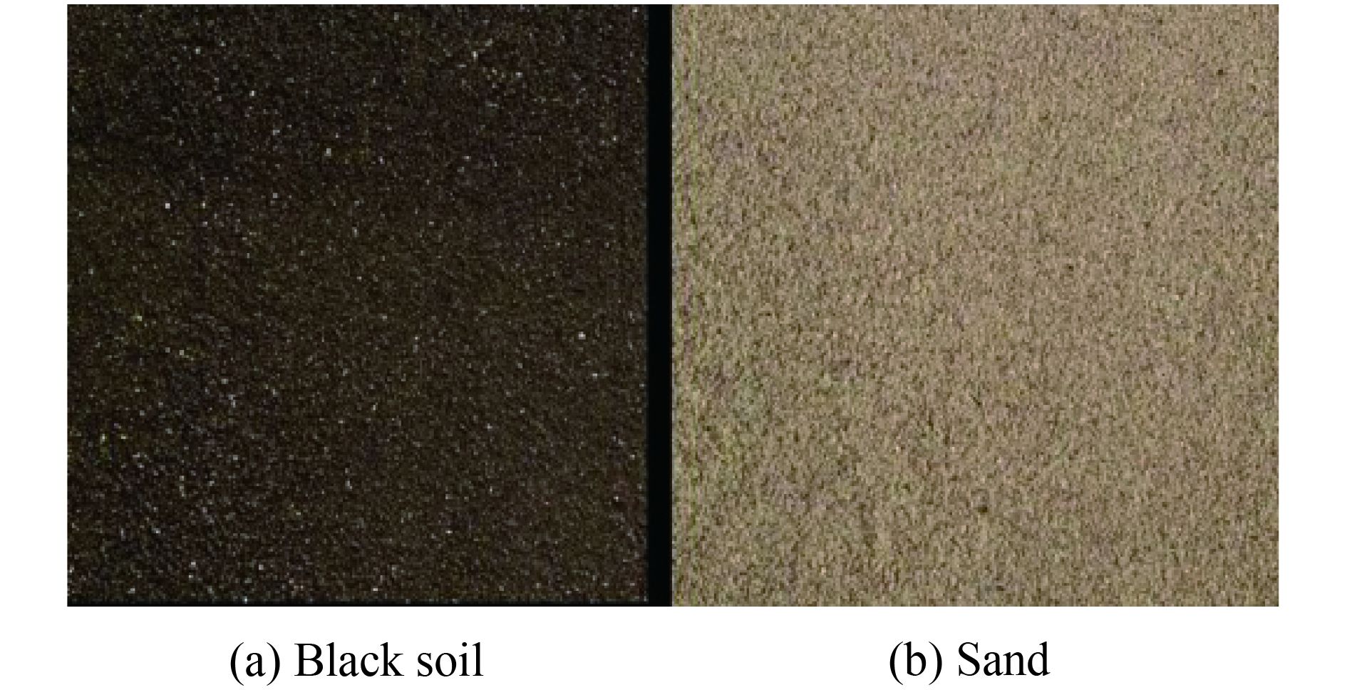
在室外天气晴朗无风的条件下，取黑土和沙土两种土壤(图6)进行实验，实验材料过20目筛子筛制而成。黑土和沙土混合方式如下(图7)，在70 cm×70 cm的纸盒中，以O为圆心，用沙土铺设半径r=15 cm的圆，其余则铺设黑土，铺设厚度约为5 cm，且土壤表面平整。

采用探头视场角为25°的FieldSpec Pro FR(Full Range)光谱仪ASD(Analytical Spectral Devices)测量混合反射光谱，在观测时，探头垂直于土壤平面，观测中心点为O，观测高度为1.2 m，根据式(1)，此时观测半径R约为26.60 cm。

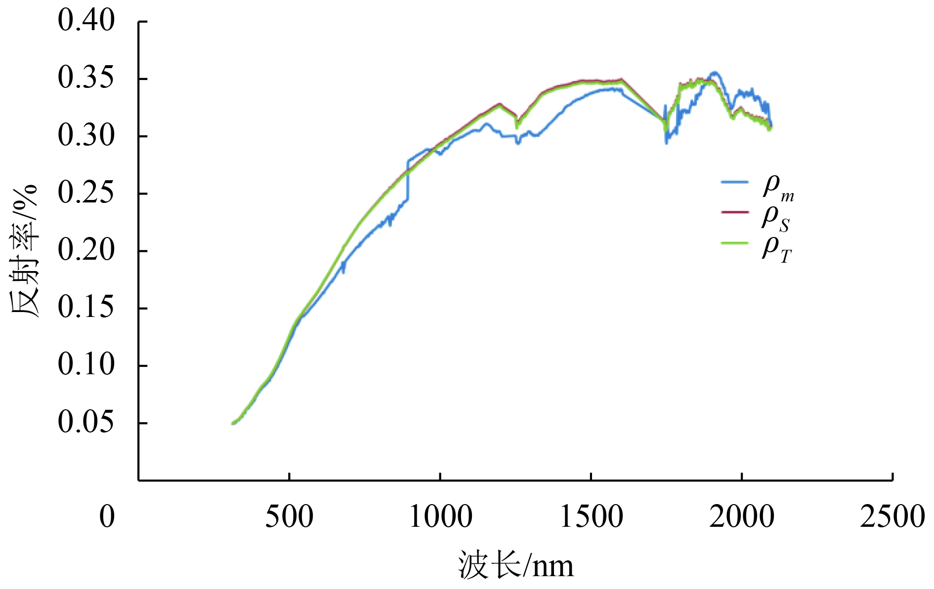
各采集5次混合反射光谱及黑土、沙土反射光谱，取其平均值进行数据分析。由于实测反射光谱数据在1351—1399 nm、1801—1949 nm和2351—2500 nm范围内波动异常，为噪声数据，故剔除。设ρ_m代表实测混合反射光谱，ρ_T和ρ_S分别代表ILSMM和LSMM的理论计算结果，根据式(13)—(16)可得

${\rho _T} = \frac{{{\rho _A}{{\sin }^2}{\beta _1} + {\rho _B}\left({{{\sin }^2}\beta - {{\sin }^2}{\beta _1}} \right)}}{{2\left({1 - \cos \beta } \right)}}$

(27)

式中，β₁为沙土边界对应的天顶角。

按照式(18)，ρ_S应为

${\rho _S} = {\rho _A}{S_A} + {\rho _B}{S_B}$

(28)

式中，ρ_A、ρ_B分别代表黑土和沙土反射率，S_A、S_B分别代表黑土和沙土的面积比。

经过计算，得到两模型的理论计算结果与实测反射光谱数据关系如下(图8)，通过比较ρ_T、ρ_S和ρ_m，结果表明，ρ_T、ρ_S均有90 %以上的数据与ρ_m的误差绝对值小于10 %，说明ρ_T、ρ_S和ρ_m有较好的一致性。

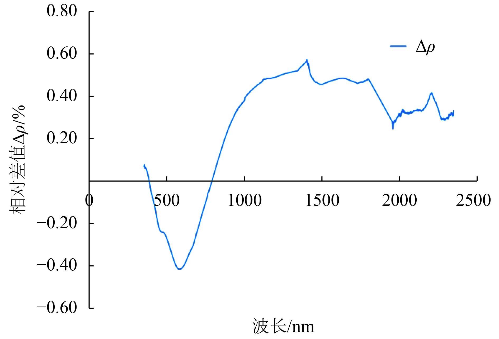
按照式(22)计算ILSMM和LSMM的相对差值Δρ(图9)，得到Δρ绝对值的最大值(|Δρ|max)小于0.6%，表明该条件下两模型的计算结果十分接近。

为研究不同的地物拓扑位置对两模型关系的是否会产生影响，通过室内实验固定两土样的面积比，改变土样的拓扑位置来进一步验证模型的适用性和准确性。

在室内实验中，设定黑土和沙土面积比为1∶1，固定观测高度为35 cm，观测中心点为O，通过以下两种不同的铺设方式(图10)来进行验证，采用光谱仪各采集5次混合反射光谱和黑土、沙土的反射光谱，并取5次测量的平均值进行分析。为使分析结果更为准确，去除了350—399 nm，1351—1399 nm、1801—1949 nm和2351—2500 nm波段范围内的噪声数据。

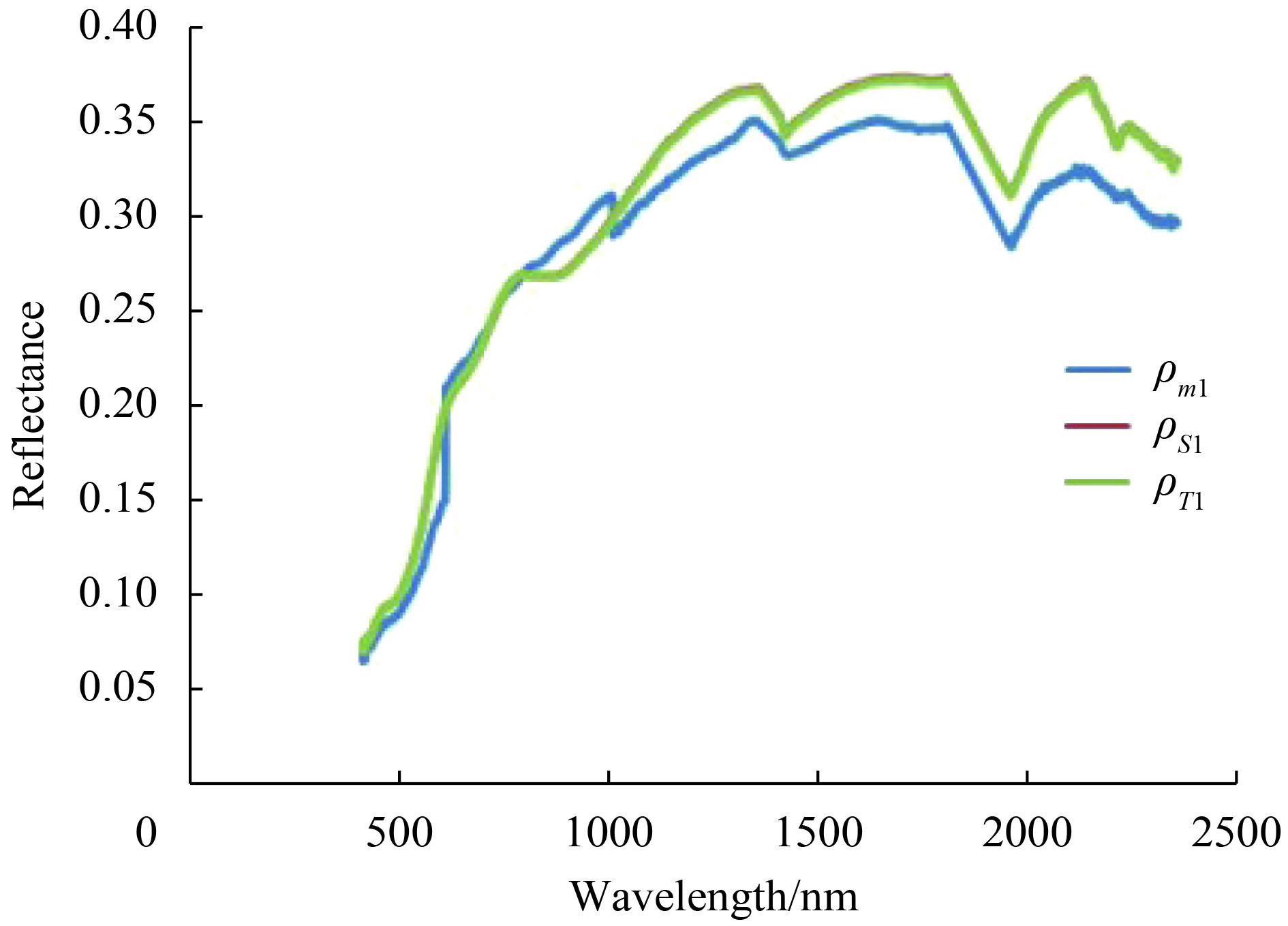
当混合方式如下(图10(1))时，记实测混合光谱、LSMM模拟结果和ILSMM的模拟结果分别为ρ_m1、ρ_S1和ρ_T1，同样，当混合方式为(图10(2))时，记实测混合光谱、LSMM模拟结果和ILSMM的模拟结果分别为ρ_m2、ρ_S2和ρ_T2，并按照式(28)、式(29)分别计算ρ_S1和ρ_S2、ρ_T1和ρ_T2。

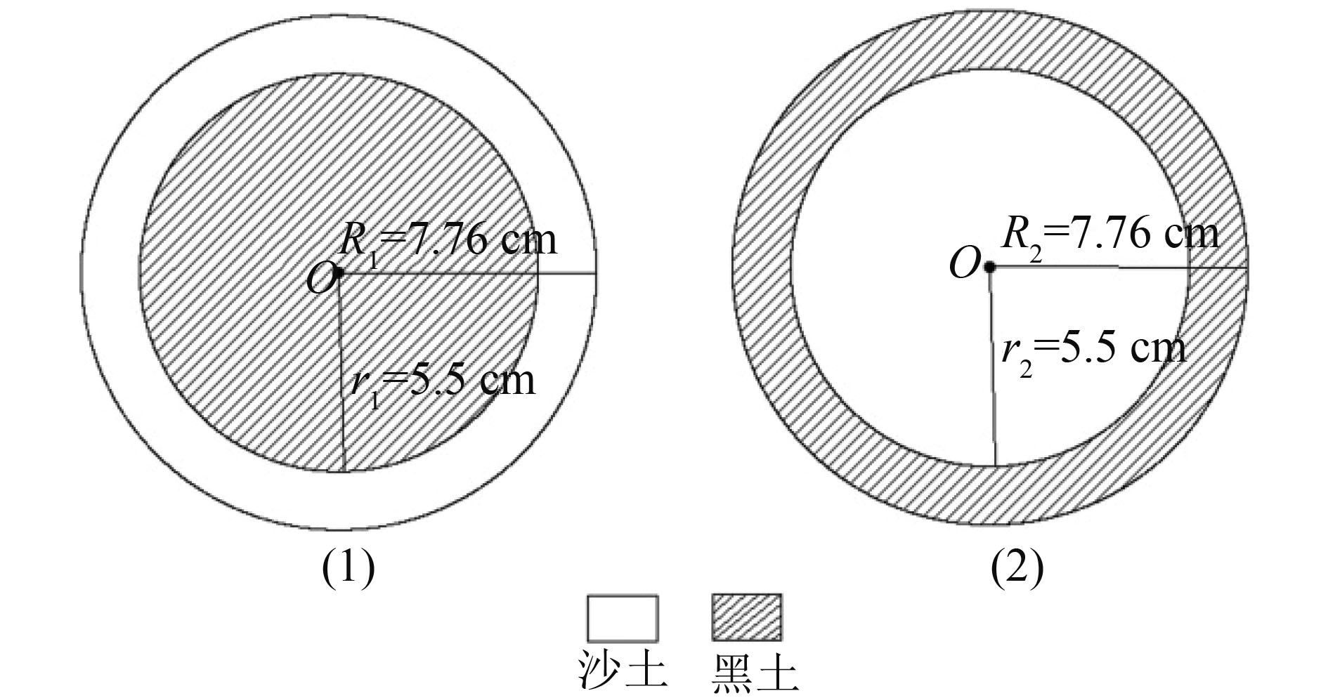
当混合方式为(图10(1))时，两模型的计算结果和实测反射光谱关系如下(图11)

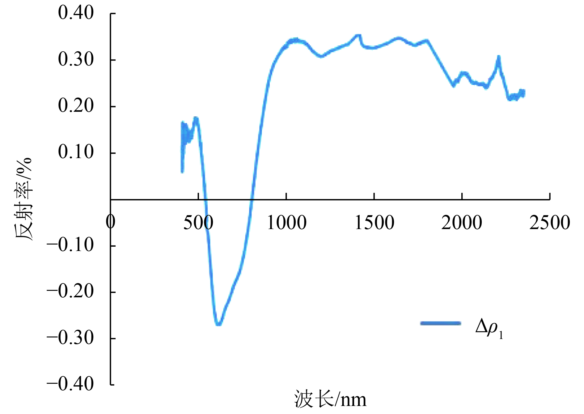
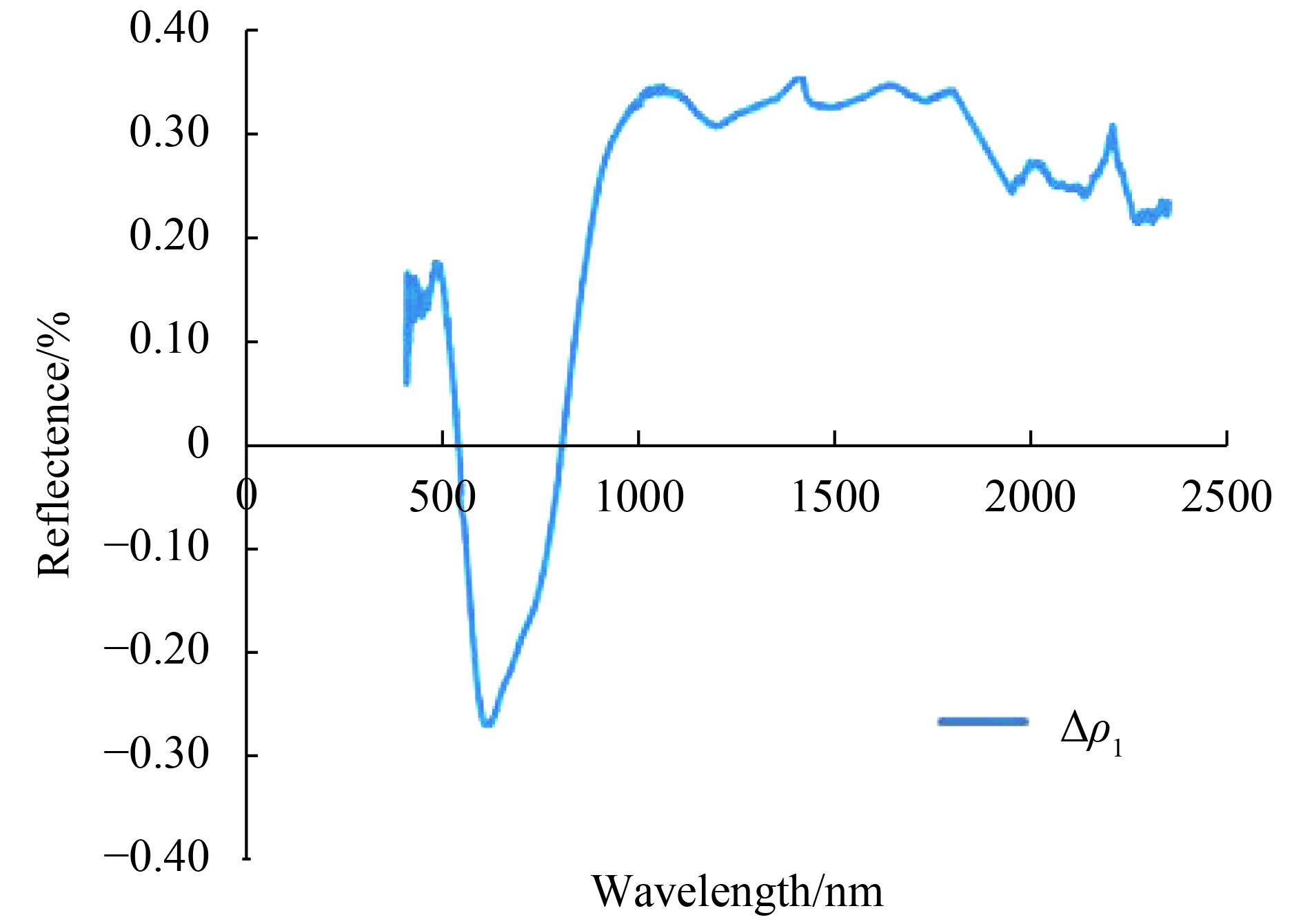
按照式(22)计算两模型相对差值Δρ₁(图12)，可得该条件下的|Δρ₁|_max小于0.4%。

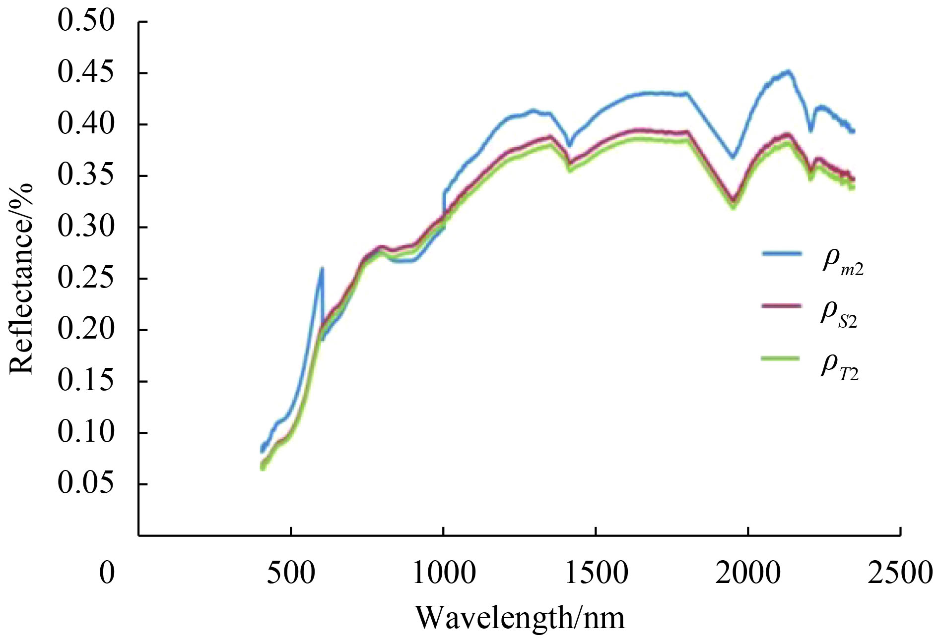
当混合方式为(图10(2))时，两模型的计算结果和实测反射光谱关系如下(图13)

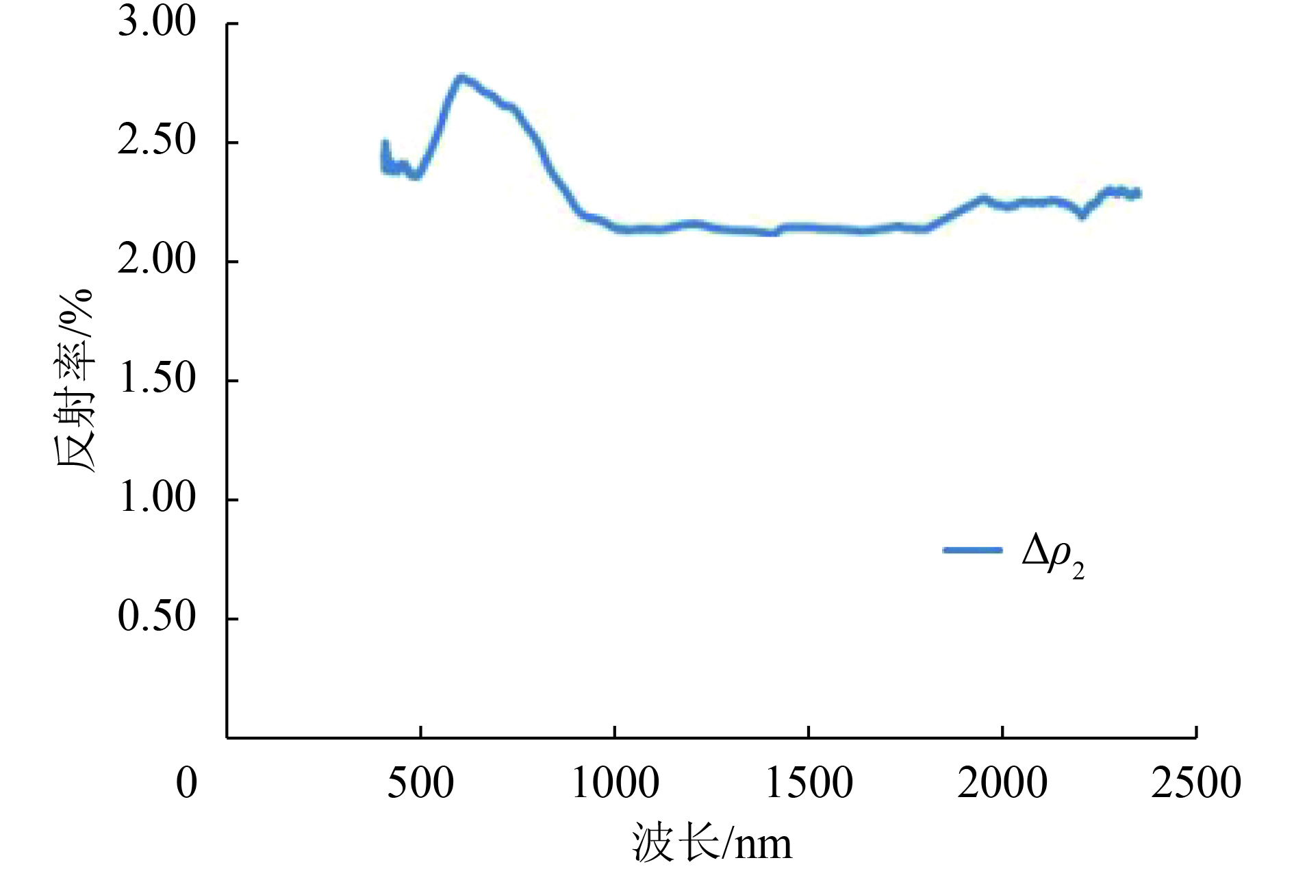
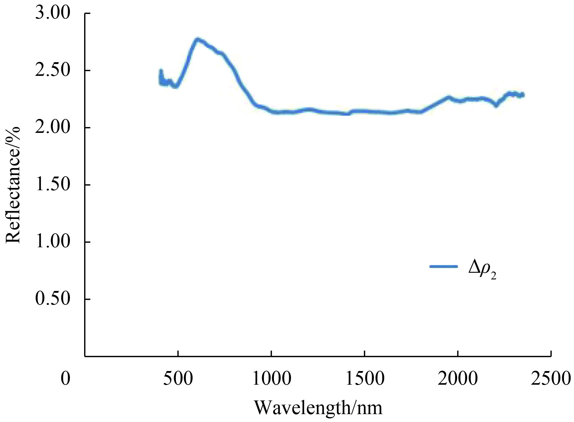
同样，按照式(22)计算两模型相对差值Δρ₂，可得该条件下|Δρ₂|_max小于3%。

通过对室外实验数据的分析可得，当β为12.5°时，即在宏观观测尺度条件下，两模型的理论计算结果均与实测混合反射光谱结果较为接近，并且LSMM和ILSMM的计算结果相近，相对差值不超0.6%，此时天顶角对混合光谱的影响可以忽略，LSMM可以代替ILSMM进行混合像元的分解。同时，室内实验结果表明，当地物面积比一定时，两模型的关系和模型的适用性不会受到地物拓扑位置的变化的影响。

线性光谱混合模型在混合像元分解中应用广泛，分析该模型的适用条件对遥感图像处理和应用有很大的实际意义。本文采用理论推导和数值模拟的方法建立了积分线性混合模型，并结合室内外实验验证，在分析ILSMM和LSMM关系的基础上得到了以下结论：

(1) 地物端元对混合光谱的影响取决于端元反射率、面积比和天顶角3个参数。其中，混合光谱是天顶角的非线性函数，在观测视域边界处天顶角的影响尤为显著。

(2) ILSMM与LSMM的相对差值Δρ仅与探测单元半瞬时视场角β有关。当观测目标为均一朗伯体时，Δρ与 ${\tan ^2}\left({\displaystyle\frac{\beta }{2}} \right)$ 为确定性关系， $\Delta \rho = {\tan ^2}\left({\displaystyle\frac{\beta }{2}} \right)$ ；当地物微面元取随机反射率时，Δρ与 ${\tan ^2}\left({\displaystyle\frac{\beta }{2}} \right)$ 具有统计关系，两者显著线性相关， $\bar \Delta \rho = 0.9993{\tan ^2}\left({\displaystyle\frac{\beta }{2}} \right)$ ，标准差和β的关系可表示为 ${S_{\Delta \rho }} = 0.0050/$ $\left[ {1/\tan{^2}\left({\displaystyle\frac{\beta }{2}} \right) - 0.7500} \right]$ 。

(3) Δρ随β的减小而减小。β<13°时，Δρ<0.0150，S_Δρ<0.0001，两模型差异极小，LSMM可视为ILSMM的近似表达，β>13°时，天顶角的影响不能忽略，Δρ逐渐增大，LSMM的适用程度逐渐降低，因此β=13°可作为大小观测尺度的分界点，β<13°时为大尺度观测，反之则为小尺度观测。

(4) 经室外实验验证，当β=12.5°时，两模型的相对差值|Δρ|_max<0.6%，表明在宏观尺度观测时，天顶角的影响可以忽略，考虑到计算的简便性，可采用LSMM进行混合像元的分解。

(5) 室内实验的结果表明ILSMM和LSMM的关系以及模型的适用性不受地物拓扑位置变化的影响。

通过以上讨论，证明了β完全可作为确定LSMM适用观测尺度的关键依据，在理论上解释了LSMM仅适用于宏观观测尺度下混合像元分解的原因，为确定线性光谱混合模型的适用观测尺度范围提供了理论依据。

遗憾的是，由于实验设备的限制，本文仅在视场角为25°的条件下进行了实验，因此在以后的工作中，文中的方法和结论还有待不同瞬时视场角下的实测光谱数据进行进一步的验证和应用。

In remote sensing observations, mixed pixels are commonly present in the observation results on account of the diversity of spectral features of surface feature and the limitation of spatial resolution of sensor (Hui et al., 2007). One of the most important obstacles to the in-depth study of quantitative remote sensing is the existence of mixed pixels (Lyu et al., 2003). In order to solve this problem, many researchers have proposed a variety of mixed pixel decomposition models which includes Linear Spectral Mixture Model (LSMM), Probability Model, Geometrical Optics Model, Stochastic Geometric Model and Fuzzy Model (Charles et al., 1996). Among these spectral mixture models above, LSMM has been widely used for its good scientific nature in theory, and straightforward physical meaning (Chen et al., 2016).

Due to the complexity of the earth’s surface and the multiple temporal and spatial resolution characteristics of remote sensing observations, the ground information acquired by remote sensing images has a large span (Li et al., 2000, 2002). Thus, there must be multi-scale problems in the geoscience description based on remote sensing (Li et al., 2013). In practical applications, it is often necessary to select the appropriate scale according to different situations (Curts E. W et al., 1987). Therefore, when describing different geologic phenomena and surface processes, the effect of scale effect must be considered (Luan et al., 2013; Chen, 1999). The remote sensing scale is mainly spatial scale, including spatial resolution and spatial scope. The research of spatial scale effect is usually divided into the following two aspects: on the one hand, the physical laws, theorems, models, and concepts of remote sensing are studied at specific scales, on the other hand, it is to analyze the variation and variation law between the parameters obtained under different observational scales or spatial resolutions (Huang et al., 2016; Wan et al., 2008).

Although the Linear Spectral Mixture Model is a simple and effective method to solve the decomposition of mixed pixels in the macroscopic observation scale, it is no longer applicable in the microscopic observation scale (Li, 2004; Liu et al., 2014). For further explore the application of Linear Spectral Mixture Model at different observation scales, firstly, based on the ground material radiation principle, the expressions of the ground surface micro facet radiant flux and the Integral Linear Spectral Mixture Model are deduced. Then the relative difference Δρ of the two models is calculated separately in the two cases of the surface features adopting uniform reflectance and the numerical simulation method generating the random reflectance. Combined with outdoor and indoor experimental measured spectral data verification, thus proving the semi-instantaneous field of view (β) can be used as the key basis for determining the applicable observational scale of Linear Spectral Mixture Model.

In mixed pixels, the endmember can be regarded as consisting of many micro-facets with the same reflectivity. The mixing spectrum at a certain wavelength should be the sum of the effective radiant energy of all micro-facets. At the beginning, the expression of the radiant flux of the micro-facet at the entry pupil of the probe is deduced. Based on this, Integral Linear Spectral Mixture Model (ILSMM) is established.

Take non-imaging spectrometer observations as an example. When the spectrometer is observed perpendicular to the horizontal ground, the observation height is represented by H, the s-IFOV of the spectrometer probe is denoted by β, A and dA respectively represent the center point and area of the probe, O is the projection of point A on the surface of the object. The observation range is a circle with O as its center and R as its radius. The following relationship exists:

$R = H\tan \beta $

(1)

It is assumed that in the spectrometer’s field of view, a certain endmember is Lambertian object and its radiance is L. There is a micro-facet on it, the center point is B and the area is dS. The angle between AO and AB (that is, the zenith angle) is θ (Fig.1).

The distance (D) between A and B can be obtained as

$D = \frac{H}{{\cos \theta }}$

(2)

The solid angle formed by point B in the direction of the spectrometer probe is (Zhao et al., 2013)

$d\varOmega = \frac{{dA\cos \theta }}{{{D^2}}} = \frac{{dA{{\cos }^3}\theta }}{{{H^2}}}$

(3)

It is assumed that at a certain wavelength, the effective radiant flux of the micro-facet in the entrance pupil of the spectrometer probe is dM. According to the definition of radiance (Zhao et al., 2013), it can be obtained

$dM = L \cdot d\varOmega \cdot dS\cos \theta $

(4)

Substituting equation (3) into equation (4) results in

$dM = L \cdot dS \cdot \frac{{dA{{\cos }^4}\theta }}{{{H^2}}}$

(5)

According to the Lambertian radiation characteristics, in the hemisphere space, the radiant exitance of this endmember is πL (Zhao et al., 2013). Assuming that the vertical incident irradiance at the surface is E, the surface features reflectivity is ρ, the formula is derived as

$\rho E = {\text{π}} L$

(6)

Substituting equation (6) into equation (5) yield

$dM = \frac{{\rho E}}{{\text{π}}} \cdot dS \cdot \frac{{dA{{\cos }^4}\theta }}{{{H^2}}}$

(7)

Combine equations (1) and (7) to get

$dM = \rho E*dS'*dA{\cos ^4}\theta {\tan ^2}\beta $

(8)

Among them, dS’ represents the area ratio of the micro-facet.

It can be seen that dM is not only influenced by the reflectivity of the endmember and the area ratio, but also has a nonlinear relationship with the zenith angle. The larger θ is the more significant is the influence on dM. In order to further analyze the relationship between the mixed spectrum and the radiant flux of micro-facet, the expression of ILSMM is deduced on the basis of the above content.

The mixed spectrum should be a linear sum of the effective radiant energies of all micro-facets within the observed horizon. To derive the expression of ILSMM, the observation range is divided into micro-facets using the following method: in the first instance make concentric circle with O as the center and R_i as the radius, where 0<R₁<R₂ $ \cdots $ < R_i< $ \cdots $ < R_n−1<R (R_i+1−R_i=dr, n→∞); after that with O as the vertex, the azimuth is equally divided into m parts in the range of 2π, where 0<φ₁<φ₂ $ \cdots $ < φ_i< $ \cdots $ < φ_m−1<2π (φ_i+1−φ_i=dφ, m→∞)(Fig.2). In this way, the observation range are divided into many fan-shaped micro-facets, the total number of micro-facets is N.

In the first place, it is assumed that the observational object is a single Lambertian object, that is, the reflectance in each place and the radiance in all directions are equal. At a certain wavelength, the radiance of the macro-facet is L_K, and the reflectivity is ρ_K. Because the reflectance is continuous and equal, the total radiant flux M_K can be obtained as

${M_K} = \iint {\frac{{{\rho _K}E}}{{\text{π}}}} \cdot dS \cdot \frac{{dA{{\cos }^4}\theta }}{{{H^2}}}$

(9)

The area of the fan arc micro-facet is (Fig. 3)

$dS = \frac{1}{2}d\varphi \left( {{{\left({r + dr} \right)}^2} - {r^2}} \right) = rdrd\varphi + \frac{1}{2}d\varphi d{r^2}$

(10)

Since dr, dφ are all small and negligible, the area of the micro-facet can be approximated as

$dS = rdrd\varphi $

(11)

And r=Htanθ, so,

$dr = \frac{H}{{{{\cos }^2}\theta }}d\theta $

(12)

Substituting equations (11) and (12) into equation (9) yields the expression for M_K as

${M_K} = \frac{{{\rho _K}E}}{{\text{π}}} \cdot dA\mathop \int \limits_0^{2{\text{π}}} d\varphi \mathop \int \limits_0^\beta \sin \theta \cos \theta d\theta $

(13)

After simplification and settlement, M_K can be obtained as

${M_K} = {\rho _K}E \cdot \sin{^2}\beta \cdot dA$

(14)

The solid angle established by the spectrometer probe over its observation range is

$\varOmega = 2{\text{π}}\left({1 - \cos \beta } \right)$

(15)

Assuming that the reflectivity of the mixed ground is ρ_T, combined with (4) and (15), the total radiant flux M_T of the ground surface measured by the spectrometer should be

${M_T} = \frac{{{\rho _T}E}}{{\text{π}}} \cdot 2{\text{π}}\left({1 - \cos \beta } \right) \cdot dA$

(16)

According to conservation of energy, the mixed reflectivity can be expressed as

${\rho _T} = \frac{{{\rho _K}{{\sin }^2}\beta }}{{2\left({1 - \cos \beta } \right)}}$

(17)

That is, if the surface reflectance is ρ_K, the actually measured ground surface reflectance should be ρ_T. In the LSMM, the reflectance of a pixel in each spectral band is expressed as a linear combination of the characteristic reflectance of its component endmembers weighted by their respective areal proportions with in the pixel (Li, 2008). Therefore, in accordance with LSMM under this condition, the mixed reflectance should be

${\rho _S} = \mathop \sum \limits_{i = 1}^N \frac{{{\rho _K}d{S_i}}}{{{\text{π}} {R^2}}} = {\rho _K}\mathop \sum \limits_{i = 1}^N \frac{{d{S_i}}}{{{\text{π}}{R^2}}}$

(18)

Obviously, the calculation result of equation (18) is ρ_K.

Equation (17) is a derivation result based on the uniform Lambertian surface. In order to derive the expression of ILSMM under normal conditions, it is assumed that the observed surface is Lambertian, and the reflectivity of each micro-facet is random value. At a certain wavelength, ρ_i, θ_i, and dS_i represent the reflectivity, corresponding zenith angle, and area of the i-th micro-facet, respectively. The sum of the radiant flux of all micro-facets should be

${M_N} = \mathop \sum \limits_{i = 1}^N {\rho _i}E \cdot dS_i' \cdot dA{\cos ^4}{\theta _i}{\tan ^2}\beta $

(19)

Combining equations (16) and (19), the general form of ILSMM can be obtained as

${\rho _T} = \frac{{{{\tan }^2}\beta }}{{2\left({1 - \cos \beta } \right)}}\mathop \sum \limits_{i = 1}^N {\rho _i}dS_i'{\cos ^4}{\theta _i}$

(20)

According to LSMM, under the above conditions, the mixed reflectivity should be

${\rho_S} = \mathop \sum \limits_{i = 1}^N {\rho _i}dS_i'$

(21)

Through the comparison of the above two cases, it is found that ILSMM and LSMM have certain similarities. Both models consider the effect of endmember reflectance and area ratio on the mixed spectrum. However, LSMM does not consider the effect of zenith angle.

For the purpose of analyze the relationship between zenith angle and mixed spectrum at different observation scales. Based on ILSMM, the relative difference Δρ between the two models is calculated according to the following formula

$\Delta \rho = \frac{{{\rho _S} - {\rho _T}}}{{{\rho _T}}}$

(22)

First, when the observation target is a single Lambertian object, Δρ can be expressed as

$\Delta \rho = {\tan ^2}\left({\frac{\beta }{2}} \right)$

(23)

Therefore, under the above conditions, there is a deterministic relationship which is $\Delta \rho = {\tan ^2}\left({\displaystyle\frac{\beta }{2}} \right)$ .

β can be used to divide the observation scale. The smaller the β, the larger the ratio of the observation height and the viewing radius and the larger the observation scale. Therefore, different observations scales can be obtained by changing the value of β. There are many kinds of land-cover types in actual observations. In order to explore the generality of the relationship between the two models, it is assumed that the area and reflectivity of each micro-facet in the observation range are all random values. Taking into account the actual situation is difficult to meet the conditions, using numerical simulation methods to further discuss.

The numerical simulation process is as follows: let the β be in the range of [1, 85], the unit is degree and the step length is 1. The observations range is divided according to Fig.2, taking n=100 and m=360. This divides the observation range into N=36, 000 fan-arc micro-facets, the reflectivity of the micro-facet is randomly generated within (0, 1). After all micro-facets take random values, calculate Δρ at each β according to equation (22). A total of 5000 sets of reflectance are simulated. Finally, the mean ( $\bar \Delta \rho $ ) and standard deviation (S_Δρ) of all Δρ at each β are calculated.

Using the linear regression model y=Kx in SPSS18.0 to perform regression analysis on $\bar \Delta \rho $ and ${\tan ^2}\left({\displaystyle\frac{\beta }{2}} \right)$ (Fig.4), the linear correlation coefficient of two variables R²=1 and the regression equation is

$\bar \Delta \rho = 0.9993\,\,{\tan ^2}\left({\frac{\beta }{2}} \right)$

(24)

Under the given reliability α=0.05, F-test is performed on the regression equation. The results show that F=1.746×10⁸, critical value F_α (1, 80)=3.96 and F>F_α, which indicated that the regression equation is valid.

Since the expression for direct derivation of S_Δρ is very complex, the relationship between β and S_Δρ is analyzed by means of curve fitting. Regression analysis is performed on ${\tan ^2}\left({\displaystyle\frac{\beta }{2}} \right)$ and S_Δρ (Fig. 5). The correlation coefficient R² is 0.9988 and fitting expression is as follows

${S_{\Delta \rho }} = 0.0050/\left( {1/\tan{^2}\left({\frac{\beta }{2}} \right) - 0.7500} \right)$

(25)

A statistical analysis is performed on 5000 sets of Δρ at each β. Plot the probability density function distribution curve and calculate the kurtosis and skewness of each curve. Compared with the normal distribution of kurtosis (b_k)=3 and skewness (s_k)=0, the kurtosis values of all distribution curves are greater than 3, and 3<b_k<5; the skewness value is 41 positive and 44 negative, 0<|s_k| <0.2. So Δ ρ presents a sharp peak distribution. To further analyze the distribution characteristics of Δρ, the standard deviation coefficient V of Δρ at each β is calculated according to the following formula (Zhou, 2001)

$V = \frac{{{S_{\Delta \rho }}}}{{\bar \Delta \rho }}$

(26)

The range of the obtained V is [0.60%, 1.34%], which indicated that the discretization of the Δρ distribution curve is very small, ${\bar \Delta \rho }$ is highly representative and the stability of the data is fine.

The available data shows that the IFOV of the aerial imaging spectrometer is generally 1.0 to 3.0 mrad, and a few are lower than 1 mrad. The aerospace imaging spectrometer includes two resolutions: medium and high resolution (Zhao et al. 2013), when the observations height is 705 km, the maximum IFOV of the MODIS is about 1.4 mrad, and the IFOV of the Hyperion is about 0.04 mrad. The above imaging spectrometer’s observations height is much larger than the observations sight radius. Therefore, the remote sensing image obtained by the aerial or space imaging spectrometer can be regarded as the observation result on the macro-scale. From the above, when the macro-scale observations are performed, the Δρ of the two models is small, so the ideal results can also be obtained by using the LSMM for the decomposition of mixed pixels. However, as the observation scale is reduced, the role of the zenith angle cannot be ignored. The difference between the two models is gradually increased, LSMM is no longer applicable. So the decomposition of the mixed pixels must be performed in accordance with ILSMM.

Under the conditions of sunny weather and no wind, the black soil and sand (Fig. 6) were taken for experiment, and the experimental materials were sieved through a 20 mesh sieve. The black soil and sand are mixed as follows (Fig. 7). In a 70 cm×70 cm carton, with O as the center, a circle with a radius of r=15 cm is laid with sand, and the rest is laid with black soil, the thickness is about 5 cm, and the soil surface is flat.

The mixed reflectance spectra were measured using a FieldSpec Pro FR (Full Range) analytical spectral devices (ASD) with a viewing angle of 25°. When observing, the probe was perpendicular to the soil plane, the observation center point was O, and the observation height was 1.2 m. According to formula (1), the observation radius at this time R is about 26.60 cm.

Five times of mixed reflection spectrum and black soil and sand reflection spectrum were collected, and the average value was taken for data analysis. Since the measured reflectance spectral data fluctuates abnormally in the range of 1351—1399 nm, 1801—1949 nm, and 2351—2500 nm, it is noise data, so it is eliminated. It is assumed that ρ_m represents the measured mixed reflection spectrum, and ρ_T and ρ_S represent the theoretical calculation results of ILSMM and LSMM, respectively, according to equations (13)—(16)

${\rho _T} = \frac{{{\rho _A}{{\sin }^2}{\beta _1} + {\rho _B}\left({{{\sin }^2}\beta - {{\sin }^2}{\beta _1}} \right)}}{{2\left({1 - \cos \beta } \right)}}$

(27)

Among them, β₁ is the zenith angle corresponding to the sand boundary.

According to equation (18), ρ_S should be

${\rho _S} = {\rho _A}{S_A} + {\rho _B}{S_B}$

(28)

Among them, ρ_A and ρ_B represent the reflectivity of black soil and sand, and S_A and S_B represent the area ratio of black soil and sand.

After calculation, the relationship between the theoretical calculation results of the two models and the measured reflectance spectral data is as follows (Fig. 8). By comparing ρ_T, ρ_S and ρ_m, the results show that within the error tolerance, the theoretical calculation results of the two models are in good agreement with the measured mixed spectra.

Calculate the relative difference Δρ of the ILSMM and LSMM according to equation (22) (Fig. 9), and obtain the maximum value of Δρ absolute value (|Δρ|_max) is less than 0.6%, which indicates that the calculation results of the two models are very close under this condition.

In order to study whether the topological position of different features affects the relationship between the two models, the area ratio of the two soil samples is fixed by indoor experiments, and the topological position of the soil samples is changed to further verify the applicability and accuracy of the model. In the indoor experiment, the black soil and sand area ratio is set to 1∶1, the fixed observation height is 35 cm, and the observation center point is O, which is verified by the following two different laying methods (Fig. 10). Five times of mixed reflection spectrum and black soil and sand reflection spectrum were collected, and the average value was taken for data analysis. In order to make the analysis more accurate, noise data in the 350—399 nm, 1351—1399 nm, 1801—1949 nm, and 2351—2500 nm bands were removed.

When the mixing method is as follows (Fig. 10(1)), the measured mixed spectrum, LSMM simulation results and ILSMM simulation results are ρ_m1, ρ_S1 and ρ_T1, respectively. Similarly, when the mixing mode is (Fig. 10(2)), it is assumed that the simulated mixed spectrum, the LSMM simulation result, and the ILSMM simulation result are ρ_m2, ρ_S2, and ρ_T2, respectively. Besides, ρ_S1 and ρ_S2, ρ_T1 and ρ_T2 are calculated according to equations (27) and (28), respectively.

When the mixing method is (Fig. 10(1)), the relationship between the calculated results of the two models and the measured reflectance spectra is as follows (Fig. 11):

Calculating the relative difference Δρ₁ of the two models according to equation (22) (Fig. 12), it is found that |Δρ₁|_max under this condition is less than 0.4%.

When the mixing method is (Fig. 10(2)), the relationship between the calculated results of the two models and the measured reflectance spectra is as follows (Fig. 13)

Similarly, the relative difference Δρ₂ of the two models is calculated according to equation (22), and |Δρ₂|_max is less than 3% under this condition.

Through the analysis of the outdoor experimental data, it can be obtained that when β is 12.5°, that is, under the condition of macroscopic observation, the theoretical calculation results of the two models are close to the measured mixed reflection spectra. The relative difference between the two models is not more than 0.6%. At this time, the influence of the zenith angle on the mixed spectrum can be neglected. LSMM can replace the ILSMM for the decomposition of mixed pixels. At the same time, the results of indoor experiments show that the relationship between the two models and the applicability of the model are not affected by changes in the topological position of the ground object when the area ratio of the objects is fixed.

The LSMM is widely used in the pixel unmixing. The analysis of the applicable conditions of the model has great practical significance for remote sensing image processing and application. In this paper, the ILSMM is established by theoretical derivation and numerical simulation. Combined with indoor and outdoor experimental verification, the following conclusions are obtained based on the analysis of the relationship between ILSMM and LSMM:

(1) The mixed spectrum is influenced by three parameters which are the reflectivity, area ratio and zenith angle of the end-members. Among these parameters, the mixed spectrum is a non-linear function of the zenith angle, in addition, the larger the zenith angle is and the more significant is the effect on the mixed spectrum.

(2) The relative difference Δρ between ILSMM and LSMM is only related to the s-IFOV (β) of the spectrometer. When observing a single Lambertian objects, the relationship between Δρ and ${\tan ^2}\left({\displaystyle\frac{\beta }{2}} \right)$ is deterministic which is $\Delta \rho = {\tan ^2}\left({\displaystyle\frac{\beta }{2}} \right)$ . When the micro-facet takes random reflectivity, Δρ has a statistical relationship with ${\tan ^2}\left({\displaystyle\frac{\beta }{2}} \right)$ which are significantly linearly related that $\bar \Delta \rho = 0.9993{\tan ^2}\left({\displaystyle\frac{\beta }{2}} \right)$ , additionally, the relationship between the standard deviation and β can be expressed as ${S_{\Delta \rho }} = 0.0050/$ $\left[ {1/\tan{^2}\left({\displaystyle\frac{\beta }{2}} \right) - 0.7500} \right]$ .

(3) Δρ decreases with the decrease of β. When β<13°, Δρ<0.0150 andS_Δρ<0.0001, the difference between the two models is very small, LSMM can be regarded as the approximate expression of ILSMM. Whenβ>13°, the influence of zenith angle cannot be ignored, Δρ gradually increases, and the applicability of LSMM gradually decreases. So β=13° can be used as the demarcation point of size observation scale, when β<13° is macroscopic observation scale, otherwise microscopic. From the above discussion, it is proved thatβ can be used as a key criterion for determining the applicable scale of LSMM. At the same time, it is theoretically explains why the LSMM is only applicable to the decomposition of mixed pixels at the macroscopic observation scale, and provides a theoretical basis for determining the range of applicable observation scales of the linear spectral mixed model.

(4) It is verified by outdoor experiments that when β=12.5°, |Δρ|_max<0.6%, indicating that the influence of zenith angle can be neglected when observed at macro scale. Considering the simplicity of the calculation, LSMM can be used to decompose the mixed pixels.

(5) The results of indoor experiments show that the relationship between ILSMM and LSMM and the applicability of the model are not affected by changes in the topological position of the features.

Through the above discussion, it is proved that β can be used as the key basis for determining the applicable measurement scale of LSMM, which theoretically explains the reason why LSMM is only suitable for the decomposition of mixed pixels in macroscopic observation scale. It provides a theoretical basis for determining the applicable measurement scale of the linear spectral mixture model.

Unfortunately, due to the limitations of the experimental equipment, the experiment was carried out only under the condition that the instantaneous field of view of 25°. Therefore, in the future work, the methods and conclusions in the paper have to be further verified and applied by the measured spectral data at different instantaneous field of views.