

|
收稿日期: 2016-11-11; 优先数字出版日期: 2018-01-01
基金项目: 国家自然科学基金(编号:41671342,U1609203,41401389);国家博士后科学基金(编号:2016T90732,2015M570668);浙江省科技厅公益技术应用项目(编号:2016C33021);宁波市自然科学基金(编号:2017A610294)
第一作者简介: 孙伟伟(1985— ),男,副教授,研究方向为地理信息系统和遥感理论和方法及“3S”技术在海岸带资源管理与环境变化监测中的应用。E-mail:sunweiwei@nbu.edu.cn
中图分类号: TP75
文献标识码: A
|
摘要
高光谱遥感影像波段众多、相关性强,导致其实际分类应用计算量大且存在明显的“维数灾难”问题。本文提出加权概率原型分析方法来研究高光谱影像的波段选择问题。该方法考虑波段间的差异性,引入综合差异性度量指标来构造权重矩阵以改进传统原型分析模型;考虑稀疏系数的狄利克雷分布和高光谱成像过程的量子特性,引入贝叶斯框架理论来构建波段选择的优化模型。加权概率原型分析方法采用迭代优化的策略,利用交替方向乘积方法来依次求解两个凸优化子问题来得到局部最优的稀疏系数矩阵并实现波段子集的最优估计。基于两个公开的高光谱数据集,对比4种主流的波段选择方法(SpaBS、SNMF、ISSC、SSR)来验证提出方法的可靠性。实验结果表明,加权概率原型分析方法的总体分类精度高于其他4种方法,能够得到更好的分类结果图。本文提出的加权概率原型分析模型能够选择合适的波段子集来满足高光谱影像的高精度分类需求。
关键词
高光谱遥感, 原型分析, 加权概率原型分析, 波段选择, 稀疏表达
Abstract
Hyperspectral imaging collects both spectral signals and images of ground objects on the Earth’s surface using hundreds of narrow bands. It has become a powerful technique for air-to-land observation. Unfortunately, numerous bands and strong intra-band correlations bring about information redundancy and heavy computational burdens for hyperspectral imagery (HSI) classification. Moreover, the " Hughes” problem traps the HSI data into a conflict between a high classification accuracy and an improbably large number of training samples. Therefore, proper bands should be selected from original hyperspectral data to reduce the high computations while achieving superior classification accuracies. In this study, a Weighted Probabilistic Archetypal Analysis (WPAA) method is proposed to extract proper bands from HSI data. WPAA considers the differences between pairwise bands and adopts a composite dissimilarity measure to construct a weighted matrix. This method improves the regular archetypal analysis by using the constructed weighted matrix in hyperspectral bands. Thereafter, the method considers the Dirichlet distribution of sparse coefficients and the quantum nature of hyperspectral imaging. It also introduces the Bayesian framework to construct its mathematical model for band selection. WPAA implements an iterative optimization scheme, transforms unconvex problems into two convex subproblems, and utilizes the Alternating Direction Method of Multipliers (ADMM) to estimate two sparse coefficient matrices. ADMM introduces proper auxiliary variables to augment the constraints in the objection function of WPAA, iteratively minimizes the Lagrangian function with respect to the primal variables, and maximizes it with respect to the Lagrange multipliers. The iteration procedure of two sparse coefficient matrices is repeated until the convergence conditions are satisfied or the number of iterations exceeds the predefined maximal number of iterations. The proper band subset is finally estimated using the sparse reconstruction equation. Two groups of classification experiments on the popular HSI datasets of PaviaU and Urban were designed to carefully test the performance of WPAA in band selection. Four state-of-the-art methods were compared against the proposed WPAA method, i.e., the sparse-based band selection, sparse nonnegative matrix factorization, improved sparse subspace clustering, and sparse self-representation. Experimental results show that WPAA achieves better overall classification accuracy than the other four state-of-the-art methods. WPAA could also obtain the best classification map regardless of the different sizes of the band subset and different training samples. The proposed composite dissimilarity weighted matrix makes great contributions to the improvement of the classification accuracy of the PAA model. WPAA could help select the proper bands for hyperspectral images, and it can serve as a good alternative for dimensionality reduction in hyperspectral image classification.
Key words
hyperspectral imagery, archetypal analysis, weighted probabilistic archetypal analysis, band selection, sparse representation
1 引 言
依赖于成像光谱仪,高光谱遥感技术能够以数十至数百个窄波段来收集地物可见光至近红外的光谱响应信息(童庆禧 等,2016;张良培和李家艺,2016)。在此基础上,通过分类来区分具有细微光谱差异的地物,对后续的植被覆盖制图、海岸带监测、矿物制图和军事目标识别等应用关系重大(杜培军 等,2016)。然而,高光谱影像数据由于波段众多,导致分类存在明显的“维数灾难”问题,需要巨大的训练样本来保证高精度的分类结果(Pal和Foody,2010)。另一方面,波段众多且相关性强,导致高光谱影像内部信息冗余较高,数据处理的计算量较大。因此,通常情况下,可以采用波段选择来进行高光谱影像数据降维,通过选取波段子集来降低数据计算量并保留重要光谱信息,然后再进行后续的高光谱影像分类处理(Sun 等,2016a, 2015b)。
近年来,稀疏表达理论的兴起,为高光谱影像的波段选择提供了新的研究思路。稀疏表达理论认为任一正常信号可以在特定字典的条件下表达为一个稀疏向量,其中少数非零元素能够很好继承原始信号的特性(Donoho,2006)。稀疏表达理论目前已经广泛应用于高光谱影像的混合像元分解(Du 等,2016)、分类(Du 等,2015)和异常探测(Zhang 等,2016)等领域。高光谱影像的稀疏系数向量能够凸显原始影像内部的一些潜在结构信息如聚类和潜在子空间等,便于实现影像的波段选择(Sun 等,2015a;张良培和李家艺,2016)。Chepushtanova等人(2014)提出稀疏支持向量机方法,利用二值支分类器来训练得到高光谱影像的各波段对应的权重,通过零和非零权重的差异来选取重要波段并得到波段子集。施蓓琦等人(2013)分析稀疏系数矩阵的聚类结构特征,利用欧氏距离度量和相对熵距离度量约束将高光谱数据矩阵分解为低阶字典矩阵和稀疏系数矩阵,根据稀疏系数矩阵中对应的系数权重大小确定该波段的聚类,最终实现波段的有效选取。Sun等人(2015b)提出改进稀疏子空间聚类方法,整合稀疏表达和子空间聚类方法,通过稀疏系数向量来构建相似性矩阵并采用谱聚类来得到合适的波段子集。最近,Sun等人(2016a)整合差异性正则项和稀疏自表达模型来构建加权差异性稀疏自表达的波段选择方法,通过非线性求解稀疏表达系数来实现波段子集的优化选择。
不同于以上方法,本文提出加权概率原型分析WPAA (Weighted Probabilistic Archetypal Analysis)方法来研究高光谱影像的波段选择问题。通过两个高光谱影像公开数据集包括Urban和Pavia University(PaviaU)进行实验分析,验证本文提出WPAA方法的有效性。
2 高光谱影像的加权概率原型分析模型
原型分析理论由Culter和Breiman(1994)提出,目前广泛应用于寻找高维数据集的代表性样本点。对于高光谱影像而言,该理论认为数据集中任一波段向量能够由其目标波段子集进行稀疏表达的线性组合来重构得到;同时,任一代表性波段可以视为由所有原始波段向量进行稀疏线性组合得到,即波段子集对应的数据点位于原始波段对应的高维数据集合所构成的凸包的边界上(Sun 等,2016a)。因此,对于高光谱影像,原型分析理论认为选取波段子集为寻找原始所有波段向量对应的高维数据点构成的最小凸包的原型点(Mørup和Hansen,2012)。假设高光谱影像构成波段集合为
| $\begin{array}{l}\quad \quad \mathop {\mathit{\boldsymbol{Y}}}\limits_{D \times N} = \mathop {\mathit{\boldsymbol{Y}}}\limits_{D \times N} \mathop {\mathit{\boldsymbol{B}}}\limits_{N \times k} \mathop {\mathit{\boldsymbol{A}}}\limits_{k \times N} + \mathop {\mathit{\boldsymbol{E}}}\limits_{D \times N} \quad \\[7pt]{\rm{s}}.{\rm{t}}.\;\left\{ \begin{array}{l}{{\mathit{\boldsymbol{b}}}_j} \geqslant 0,\;{{\mathit{\boldsymbol{b}}}_{jj}} = 0,\left| {{\mathit{\boldsymbol{b}}_j}} \right| = 1,\forall j \in \left\{ {1, \cdot \cdot \cdot ,k} \right\}\\[5pt]{{\mathit{\boldsymbol{a}}}_i} \geqslant 0\;\text{且}\;\left| {{{\mathit{\boldsymbol{a}}}_i}} \right| = 1,\forall i \in \left\{ {1, \cdots ,N} \right\}\end{array} \right.\,\end{array}$ | (1) |
式中,
常规的原型分析模型通过选取原型点来估计最佳波段子集时,并未考虑到高光谱影像不同波段的差异性导致的原型点选取时的优先度问题。波段选择的目的为选择信息量大且相关性较小的波段,因此本文采用综合差异度量CDM(Composite Dissimilarity Measure)来描述不同波段之间的综合差异,改进原型分析模型用于高光谱影像的波段选择结果(Sun 等,2016a)。综合差异性度量整合光谱信息差异性和波段相关性指标来综合评价不同波段的差异大小。假设任意两个波段向量
| ${\bf{CD}}{{\bf{M}}_{ij}} = \frac{{{\rm{SID}}({{\mathit{\boldsymbol{y}}}_i},{{\mathit{\boldsymbol{y}}}_j})}}{{R({{\mathit{\boldsymbol{y}}}_i},{{\mathit{\boldsymbol{y}}}_j})}}$ | (2) |
| ${\rm{SID}}({{\mathit{\boldsymbol{y}}}_i},{{\mathit{\boldsymbol{y}}}_j}) = {\rm{KLD}}( {{{\mathit{\boldsymbol{y}}}_i}} || {{\mathit{\boldsymbol{y}}}_j}) + {\rm{KLD}}( {{{\mathit{\boldsymbol{y}}}_j}} || {{\mathit{\boldsymbol{y}}}_i})$ | (3) |
| $R({{\mathit{\boldsymbol{y}}}_i},{{\mathit{\boldsymbol{y}}}_j}) = \frac{{\sum\limits_{l = 1}^N {({a_{il}} - {{\bar y}_i})({a_{jl}} - {{\bar y}_j})} }}{{\sqrt {\sum\limits_{l = 1}^N {{{({a_{il}} - {{\bar y}_i})}^2}} \sum\limits_{l = 1}^N {{{({a_{jl}} - {{\bar y}_j})}^2}} } }}$ | (4) |
式中,
| $\begin{array}{l}\mathop {\mathit{\boldsymbol{Y}}}\limits_{D \times N} = \mathop {\mathit{\boldsymbol{Y}}}\limits_{D \times N} \mathop {\mathit{\boldsymbol{W}}}\limits_{N \times N} \mathop {\mathit{\boldsymbol{B}}}\limits_{N \times k} \mathop {\mathit{\boldsymbol{A}}}\limits_{k \times N} + \mathop {\mathit{\boldsymbol{E}}}\limits_{D \times N} \quad \\{\rm{s}}.{\rm{t}}.\;\left\{ \begin{array}{l}{{\mathit{\boldsymbol{b}}}_j} \geqslant 0,\;{{\mathit{\boldsymbol{b}}}_{jj}} = 0,\left| {{{\mathit{\boldsymbol{b}}}_j}} \right| = 1,\forall j \in \left\{ {1, \cdot \cdot \cdot ,k} \right\}\\{\mathit{\boldsymbol{a}}_i} \geqslant 0\;\text{且}\;\left| {{{\mathit{\boldsymbol{a}}}_i}} \right| = 1,\forall i \in \left\{ {1, \cdot \cdot \cdot ,N} \right\}\end{array} \right.\,\end{array}$ | (5) |
式中,稀疏系数矩阵B和A均未知,是典型的盲信号矩阵分解问题。差异性矩阵通过权重稀疏来综合考虑不同波段的信息量和相关性,避免加权原型分析选择较为相近的波段,更有利于选择信息量大且相关性较小的波段子集。贝叶斯框架考虑光谱的空间变异性,能够将矩阵分解问题(5)转换为基于概率模型的贝叶斯预测问题。贝叶斯框架较为灵活,能够整合波段和光谱信号的先验概率分布知识,同时附加各类范数约束条件如稀疏系数矩阵B和A的非负和一阶范数为1的限制条件来保证优化结果能够得到合理解释(Bioucas-Dias 等,2012;He 等,2016)。得到加权概率原型分析模型
| $\begin{aligned}& P(\mathit{\boldsymbol{\varTheta ,B,A}}\left| {\mathit{\boldsymbol{Y}}} \right.) = \frac{{P({\mathit{\boldsymbol{Y}}}\left| {\mathit{\boldsymbol{\varTheta }},\mathit{\boldsymbol{B}},\mathit{\boldsymbol{A}}} \right.)P(\mathit{\boldsymbol{\varTheta }})P(\mathit{\boldsymbol{B}})P(\mathit{\boldsymbol{A}})}}{{P(\mathit{\boldsymbol{Y}})}}\\& \quad \quad \quad \;\; \propto P(\mathit{\boldsymbol{Y}}\left| {\mathit{\boldsymbol{\varTheta }},\mathit{\boldsymbol{B}},\mathit{\boldsymbol{A}}} \right.)P(\mathit{\boldsymbol{B}})P(\mathit{\boldsymbol{A}})\\& {\rm{s}}.{\rm{t}}.\;\left\{ \begin{array}{l}{\mathit{\boldsymbol{b}}_j} \geqslant 0,\;{\mathit{\boldsymbol{b}}_{jj}} = 0,\left| {{\mathit{\boldsymbol{b}}_j}} \right| = 1,\forall j \in \left\{ {1, \cdot \cdot \cdot ,k} \right\}\\[5pt]{\mathit{\boldsymbol{a}}_i} \geqslant 0\;\text{且}\;\left| {{\mathit{\boldsymbol{a}}_i}} \right| = 1,\forall i \in \left\{ {1, \cdot \cdot \cdot ,N} \right\}\end{array} \right.\end{aligned}$ | (6) |
式中,
| $\begin{array}{l}\mathop {\arg \max }\limits_{B,A} P(\mathit{\boldsymbol{\varTheta }},\mathit{\boldsymbol{B}},\mathit{\boldsymbol{A}}\left| \mathit{\boldsymbol{Y}} \right.)\\ = \mathop {\arg \min }\limits_{B,A} - ({\rm{lg}}P(\mathit{\boldsymbol{Y}}\left| {\mathit{\boldsymbol{\varTheta }},\mathit{\boldsymbol{B}},\mathit{\boldsymbol{A}}} \right.) + {\rm{lg}}P(\mathit{\boldsymbol{B}}) + P(\mathit{\boldsymbol{A}}))\\{\rm{s}}.{\rm{t}}.\;\left\{ \begin{array}{l}{\mathit{\boldsymbol{b}}_j} \geqslant 0,\;{\mathit{\boldsymbol{b}}_{jj}} = 0,\left| {{\mathit{\boldsymbol{b}}_j}} \right| = 1,\forall j \in \left\{ {1, \cdot \cdot \cdot ,k} \right\}\\{\mathit{\boldsymbol{a}}_i} \geqslant 0\;\text{且}\;\left| {{\mathit{\boldsymbol{a}}_i}} \right| = 1,\forall i \in \left\{ {1, \cdot \cdot \cdot ,N} \right\}\end{array} \right.\end{array}$ | (7) |
式中,lg(·)为对数运算符,
3 基于加权概率原型分析的高光谱影像波段选择
3.1 加权概率原型分析模型的求解
考虑到高光谱遥感的光学成像的量子特性,本文采用泊松分布来描述光谱的概率密度分布
| $\begin{array}{l}{\rm{argmin}}\left( {\sum\limits_{i = 1}^D {\sum\limits_{j = 1}^N {\left[ { - {{(\mathit{\boldsymbol{Y}})}_{ij}}\lg {{(\mathit{\boldsymbol{\varTheta BA}})}_{ij}}} \right.} } } \right. +\\\;\;\;\;\;\;\;\;\left. {\left. { {{\left( {\mathit{\boldsymbol{\varTheta BA}}} \right)}_{ij}} + {\rm{\lg}} {{\left( \mathit{\boldsymbol{Y}} \right)}_{ij}}!} \right]} \right)\\\;\;\;\;\;\;\;\;\;\;{\rm{s}}.{\rm{t}}.{\rm{diag}}(\mathit{\boldsymbol{B}}) = 0\end{array}$ | (8) |
假设
| $\begin{array}{l}\mathop {\arg \min }\limits_{B,A} < \mathit{\boldsymbol{\varTheta BA}} - \mathit{\boldsymbol{Y}} \circ \lg (\mathit{\boldsymbol{\varTheta BA}}),\mathit{\boldsymbol{1}} > + C\\{\rm{s}}.{\rm{t}}.{\rm{diag}}(\mathit{\boldsymbol{B}}) = 0\end{array}$ | (9) |
式中,
| $\begin{array}{l}\mathop {\arg \min }\limits_{\hat B} < \mathit{\boldsymbol{\varTheta B}}{\mathit{\boldsymbol{A}}^{(t)}} - \bf{Y} \circ \lg (\mathit{\boldsymbol{\varTheta B}}{\mathit{\boldsymbol{A}}^{(t)}}),{\bf{1}} > \;\\{\rm{s}}.{\rm{t}}.,{\rm{diag}}(\mathit{\boldsymbol{B}}) = 0\end{array}$ | (10) |
| $\mathop {\arg \min }\limits_{\hat A} < \mathit{\boldsymbol{\varTheta }}{\mathit{\boldsymbol{B}}^{(t + 1)}}\mathit{\boldsymbol{A}} - \mathit{\boldsymbol{Y}} \circ \lg (\mathit{\boldsymbol{\varTheta }}{\mathit{\boldsymbol{B}}^{(t + 1)}}\mathit{\boldsymbol{A}}),{\bf{1}} > $ | (11) |
本文采用交替方向乘积方法(Sun 等,2015b)来分别求解上述两个凸优化子问题,通过引入适当的辅助变量来增强上述约束条件,依次最小化主要变量和拉格朗日乘积构成的目标函数方程来得到局部最优解。当目标残差满足
3.2 基于WPAA的高光谱影像波段选择流程
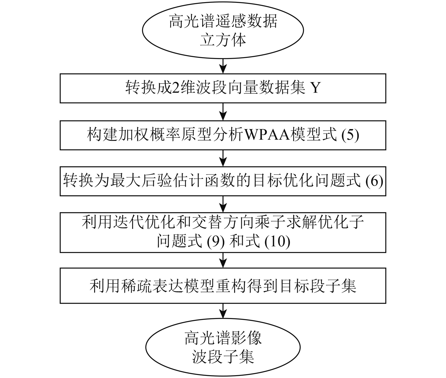
基于加权概率原型分析WPAA的高光谱影像波段选择的流程如图1。
流程中包含以下步骤:
(1) 将3维的高光谱影像立方体转换为2维波段向量数据集Y,以2维矩阵形式表示,其中波段数D为Y对应的矩阵的列数,像素个数N为Y的行数;
(2) 利用式(6)构建加权概率原型分析模型,并通过联合概率密度最大化来得到基于最大后验估计函数的目标优化问题式(7);
(3) 利用迭代优化的策略来分解问题式(7)为两个凸优化子问题式(10)和式(11),采用交替方向乘积方法来求解得到局部最优的稀疏系数矩阵
(4)利用稀疏重构表达式

4 实验与分析
4.1 实验数据
PaviaU数据来自西班牙巴斯克大学计算智能课题组(http://www.ehu.es/ccwintco/index.php/Hyper spectral_Remote_Sensing_Scenes [2016-10-11]),影像覆盖帕维亚大学区域,共103波段,空间分辨率为1.3 m(图2)。影像为较大数据集中的一部分,包含350×340像素,波段数为103,包含9类地物(包括阴影)。数据中各地物样本的真实空间分布信息如表1所示。Urban数据从美国陆军地理空间中心获取的HYDICE高光谱影像数据(http://www.erdc.usace.army.mil/Media/FactSheets/FactSheetArticleView/tabid/9254/Article/610433/hypercube.aspx[2016-10])。数据采集于1995年10月,空间分辨率为2 m,光谱分辨率为10 nm。影像大小为307×307像素,覆盖美国德克萨斯州科帕拉斯区域(靠近胡德堡)(图3)。对原始的210波段数据进行预处理,移除低噪比波段,剩余162波段,包含22种主要地物,各地物的真实分布样本信息如表2。

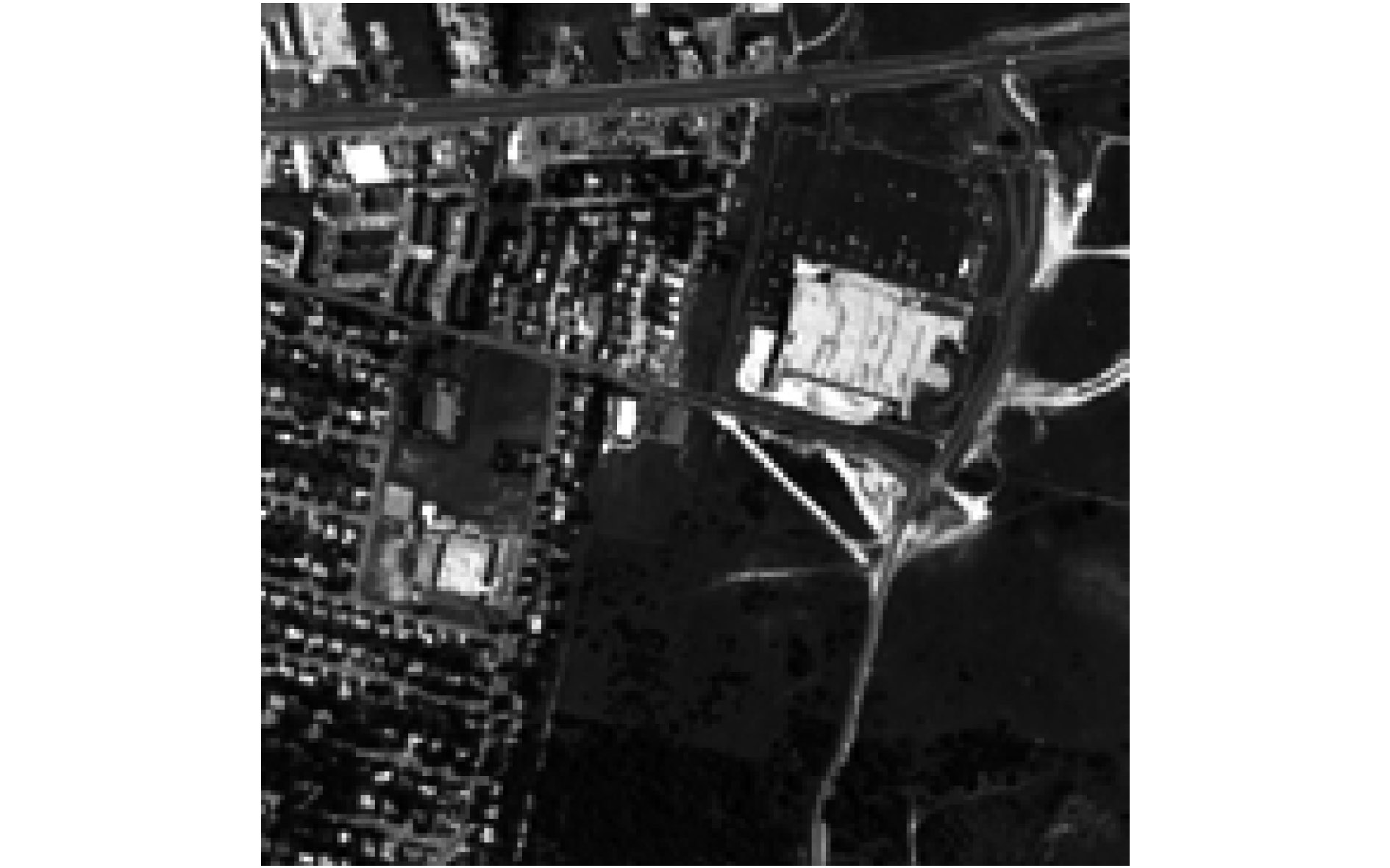
表 1 PaviaU数据的地物真实样本信息
Table 1 Ground truth of all classes of ground objects on PaviaU dataset
| 类号 | 类名 | 样本数 | 类号 | 类名 | 样本数 | |
| 1 | Asphalt | 4195 | 6 | Bare Soil | 5029 | |
| 2 | Meadows | 2185 | 7 | Bitumen | 1330 | |
| 3 | Gravel | 2099 | 8 | Self-Blocking Bricks | 2347 | |
| 4 | Trees | 1550 | 9 | Shadows | 929 | |
| 5 | Painted metal sheets | 1345 | 总数 | 20289 | ||
表 2 Urban数据的地物真实样本信息
Table 2 The ground truth of samples in each class for Urban dataset
| 类号 | 类名 | 样本数 | 类号 | 类名 | 样本数 | |
| 1 | AsphaltDrk | 85 | 13 | Roof03LgtGray | 35 | |
| 2 | AsphaltLgt | 58 | 14 | Roof04DrkBrn | 84 | |
| 3 | Concrete01 | 124 | 15 | Roof05AChurch | 85 | |
| 4 | VegPasture | 236 | 16 | Roof06School | 64 | |
| 5 | VegGrass | 127 | 17 | Roof07Bright | 72 | |
| 6 | VegTrees01 | 263 | 18 | Roof08BlueGrn | 45 | |
| 7 | Soil01 | 113 | 19 | TennisCrt | 96 | |
| 8 | Soil02 | 53 | 20 | ShadedVeg | 40 | |
| 9 | Soil03Drk | 59 | 21 | ShadedPav | 64 | |
| 10 | Roof01Wal | 118 | 22 | VegTrees01 | 261 | |
| 11 | Roof02A | 91 | 总数 | 2212 | ||
| 12 | Roof02BGvl | 39 |
4.2 实验分析
本节利用公开高光谱影像数据集PaviaU和Urban来设计3组实验以验证提出的WPAA用以波段选择的效果。实验采用支持向量机分类器SVM(Support Vector Machine)和K—近邻分类器KNN(K-Nearest Neighbor)来分类波段子集,采用总体分类精度OCA(Overall Classification Accuracy)来定量评价分类效果。SVM分类器采用径向基核函数,其方差和惩罚因子通过交叉验证获得,KNN分类器得邻域大小设定为3。从每个数据集的训练和测试样本中随机抽取10次进行实验,以下是10次独立实验的平均结果。
(1) 综合差异性权重矩阵对WPAA的贡献度分析。本实验对比分析综合差异性权重矩阵W对改进WPAA的贡献度大小。对比方法包括未包含综合差异性权重矩阵的概率原型分析方法PAA(Probabilistic Archetypal Analysis),基于综合差异性指标的波段选择方法(CDM)和本文提出的WPAA。考虑到波段选择目的为得到高光谱信息量、低波段相关性且类间差异大的波段子集,实验采用3种量化指标包括平均信息熵AIE(Average Information Entropy)、平均相关系数ACC(Average Correlation Coefficient)和平均相对熵ARE(Average Relative Entropy)分别来估计波段子集的光谱信息丰富程度,波段相关关系和波段子集的类间差异性。实验中,PaviaU和Urban数据的波段子集大小k分别人为设定为20和40。
表 3 不同波段选择方法的定量评价和分类精度对比
Table 3 The contrast in quantitative evaluation and classification accuracy from different band selection methods
| 数据 | 方法 | 定量评价指标 | 分类器 | |||
| SVM | KNN | |||||
| AIE | ACC | ARE | OCA | OCA | ||
| PaviaU (k=20) | PAA | 12.643 | 0.569 | 1.982 | 0.918 | 0.851 |
| CDM | 10.541 | 0.621 | 1.022 | 0.894 | 0.825 | |
| WPAA | 16.860 | 0.526 | 3.254 | 0.956 | 0.915 | |
| Urban (k=40) | PAA | 8.682 | 0.669 | 10.386 | 0.952 | 0.925 |
| CDM | 7.841 | 0.724 | 6.575 | 0.915 | 0.906 | |
| WPAA | 12.524 | 0.582 | 14.067 | 0.986 | 0.968 | |
表3展示PAA、CDM和WPAA在PaviaU和Urban数据集上的定量评价和分类结果。可以看出,PAA方法得到的定量评价指标和分类精度OCA都优于CDM而低于WPAA。3种方法中,WPAA方法在各方面表现最优,能够得到光谱信息量更丰富、波段相关性更小且类间差异性更大的波段子集。这说明通过引入综合差异性权重矩阵到PAA模型中,构建的WPAA模型能够明显提升CDM和PAA的波段选择结果,得到更好的高光谱影像分类结果。因此,综合差异性权重矩阵对保证WPAA的波段选择结果具有重要贡献。
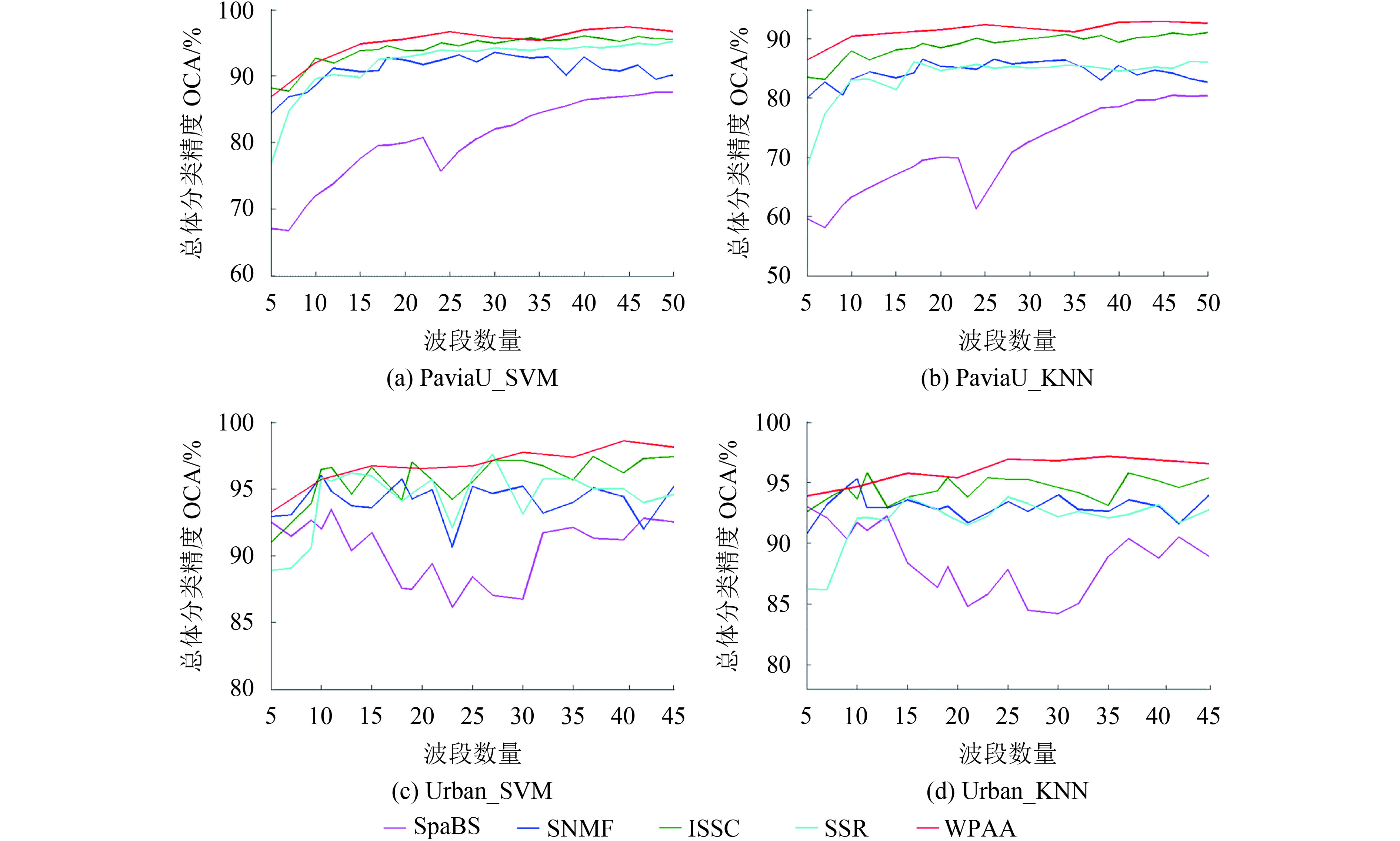
(2) 不同波段数量下的分类结果对比。本实验对比分析不同波段子集大小条件下WPAA和主流对比方法在PaviaU和Urban数据集的分类性能。采用的4种主流对比方法包括基于稀疏的波段选择法SpaBS(Sparse based band selection) (Li和Qi,2011)、稀疏矩阵分解的波段选择法SNMF(Sparse Nonnegative Matrix Factorization) (Li和Qian,2011)、改进稀疏子空间聚类方法ISSC(Improved Sparse Subspace Clustering) (Sun 等,2015b)和稀疏自表达的波段选择方法SSR(Sparse Self Representation) (Elhamifar 等,2012)。
实验中,PaviaU数据集中波段数的选择区间为5—50,Urban数据集中波段数的选择区间为4—45,步长都为5。实验选定每一类地物中20%的真实样本作为训练样本大小来进行分类实验,其余的地物样本作为测试样本。其中PaviaU和Urban数据集中,SpaBS方法的迭代次数设置为5次。利用交叉验证方法,PaviaU数据集中,SNMF方法的正则化因子α和β分别设定为4.0和1.5;Urban数据集中,SNMF方法中正则化因子α和β分别设定为3.5和0.05。
图4展示不同波段子集大小条件下的WPAA和4种对比方法在PaviaU和Urban数据集上的总体分类精度OCA曲线。可以看出,随着波段数量从5增加,5种方法的总体分类精度OCA总体上升。其中,SpaBS的OCA曲线表现最差,较不稳定,明显低于WPAA和其他方法。ISSC方法优于SNMF、SSR和SpaBS,但整体低于WPAA的OCA曲线结果。SNMF和SSR的OCA曲线结果较为接近,都明显优于SpaBS。因此,WPAA在不同波段数量条件下得到的OCA曲线表现最优,分类精度最高。
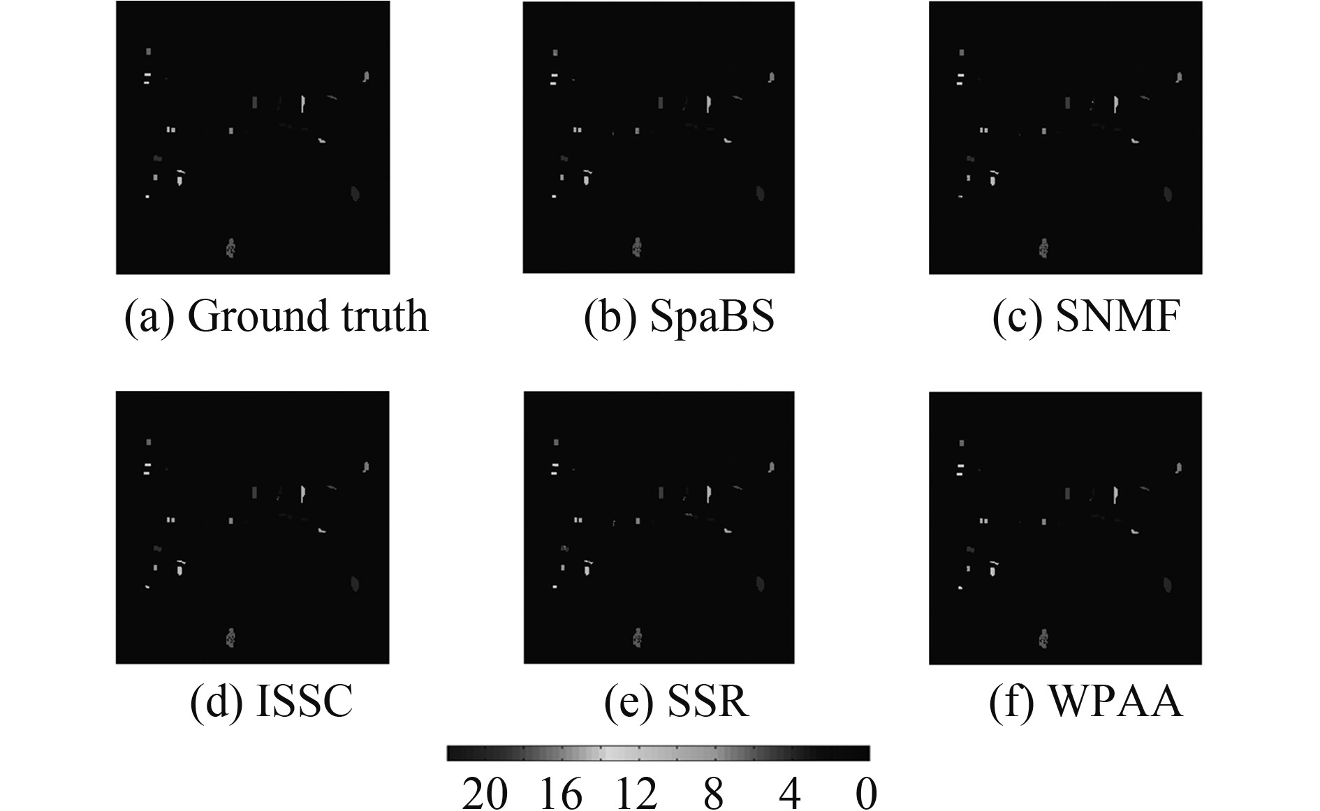
进一步,图5和图6展示WPAA和其他4种方法在选定波段子集数量条件下的分类结果。其中,PaviaU数据中波段子集k的大小为20,Urban数据集中波段子集k的大小为40。可以看出,WPAA的分类图结果优于其他4种方法。

(3) 不同训练样本大小下的分类结果对比。本实验对比分析不同训练样本条件下WPAA和其他4种对比方法(SpaBS、SNMF、ISSC和SSR)的分类结果。其中,PaviaU和Urban数据的训练样本随机采样于地物真实样本集,采样比率的选择区间为[0.05, 0.08, 0.1, 0.13, 0.15, 0.18, 0.2, 0.25, 0.3, 0.4, 0.5]。PaviaU数据中,波段数量k设定为20;Urban数据中,波段数量k设定为40。IKSSR和其他4种波段选择方法的其他参数设置都与实验(1)保持一致。

图7为不同地物训练样本大小条件下的5种方法在PaviaU和Urban数据中得到的总体分类精度OCA曲线结果。考虑到SVM和KNN分类结果趋势的一致性,图7仅列出SVM的分类结果。可以看出,随着单一地物训练样本大小的增加,各种波段选择方法得到的分类结果提升较为明显。对于任一高光谱数据集,WPAA得到的总体分类精度OCA始终高于其他4种方法包括SpaBS、SNMF、ISSC和SSR。类似于实验(1),SpaBS得到的总体分类精度OCA明显低于其他方法。SNMF和SSR的分类精度较为接近,但两者的OCA曲线低于ISSC的OCA结果。ISSC的OCA曲线高于SpaBS、SNMF和SSR,但低于WPAA方法。因此,WPAA在不同训练样本条件下得到的总体分类精度OCA最高,优于其他4种对比波段选择方法。
5 结 论
本文提出加权概率原型分析WPAA方法来解决高光谱影像的波段选择问题。WPAA方法能够考虑波段之间的差异性和高光谱遥感成像的量子特性,引入贝叶斯框架理论和波段权重矩阵来改进传统的原型分析模型。整合WPAA方法采用迭代优化的策略来转换非凸优化问题,运用交替方向乘积方法来求解得到局部最优的稀疏系数矩阵来得到合适的波段子集。利用PaviaU和Urban两个公开高光谱数据集,对比SpaBS、SNMF、ISSC和SSR 4种波段选择方法来验证WPAA的波段选择效果。实验结果表明,引入的综合差异性权重矩阵对保证WPAA的波段选择结果具有非常重要的作用。另一方面,不同波段子集和不同训练样本下的WPAA的OCA曲线都高于4种主流方法,展现其波段子集用于高光谱影像的更高精度分类的能力。因此,WPAA能够选择适合高光谱影像的波段子集,更好满足分类的应用需求。然而,本文的研究结果需要下一步的工作来进行完善和优化。在后续的工作中将考虑采用泊松分布来模拟噪声的概率分布来优化WPAA的波段选择结果。同时,将考虑采用波段高维空间分布的图谱理论来改进WPAA模型,提升WPAA的波段选择效果来满足实际高光谱影像数据处理需求。
参考文献(References)
-
Bioucas-Dias J M, Plaza A, Dobigeon N, Parente M, Du Q, Gader P and Chanussot J. 2012. Hyperspectral unmixing overview: geometrical, statistical, and sparse regression-based approaches. IEEE Journal of Selected Topics in Applied Earth Observations and Remote Sensing, 5 (2): 354–379. [DOI: 10.1109/JSTARS.2012.2194696]
-
Chepushtanova S, Gittins C and Kirby M. 2014. Band selection in hyperspectral imagery using sparse support vector machines//Procedings of SPIE 9088, Algorithms and Technologies for Multispectral, Hyperspectral, and Ultraspectral Imagery XX, 90881F. Baltimore, Maryland, USA: SPIE: 90881F [DOI: 10.1117/12.2063812]
-
Cutler A and Breiman L. 1994. Archetypal analysis. Technometrics, 36 (4): 338–347. [DOI: 10.1080/00401706.1994.10485840]
-
Dobigeon N, Tourneret J Y, Richard C, Bermudez J C M, McLaughlin S and Hero A O. 2014. Nonlinear unmixing of hyperspectral images: models and algorithms. IEEE Signal Processing Magazine, 31 (1): 82–94. [DOI: 10.1109/MSP.2013.2279274]
-
Donoho D L. 2006. Compressed sensing. IEEE Transactions on Information Theory, 52 (4): 1289–1306. [DOI: 10.1109/TIT.2006.871582]
-
Du B, Wang S D, Wang N, Zhang L F, Tao D C and Zhang L F. 2016. Hyperspectral signal unmixing based on constrained non-negative matrix factorization approach. Neurocomputing, 204 : 153–161. [DOI: 10.1016/j.neucom.2015.10.132]
-
Du P J, Xue Z H, Li J and Plaza A. 2015. Learning discriminative sparse representations for hyperspectral image classification. IEEE Journal of Selected Topics in Signal Processing, 9 (6): 1089–1104. [DOI: 10.1109/JSTSP.2015.2423260]
-
Du P J, Xia J S, Xue Z H, Tan K, Su H J and Bao R. 2016. Review of hyperspectral remote sensing image classification. Journal of Remote Sensing, 20 (2): 236–256. [DOI: 10.11834/jrs.20165022] ( 杜培军, 夏俊士, 薛朝辉, 谭琨, 苏红军, 鲍蕊. 2016. 高光谱遥感影像分类研究进展. 遥感学报, 20 (2): 236–256. [DOI: 10.11834/jrs.20165022] )
-
Elhamifar E, Sapiro G and Vidal R. 2012. See all by looking at a few: sparse modeling for finding representative objects//Proceedings of 2012 IEEE Conference on Computer Vision and Pattern Recognition. Providence, RI, USA: IEEE: 1600–1607 [DOI: 10.1109/CVPR.2012.6247852]
-
He W, Zhang H Y, Zhang L P and Shen H F. 2016. Total-variation-regularized low-rank matrix factorization for hyperspectral image restoration. IEEE Transactions on Geoscience and Remote Sensing, 54 (1): 178–188. [DOI: 10.1109/TGRS.2015.2452812]
-
Li J M and Qian Y T. 2011. Clustering-based hyperspectral band selection using sparse nonnegative matrix factorization. Journal of Zhejiang University SCIENCE C, 12 (7): 542–549. [DOI: 10.1631/jzus.C1000304]
-
Li S J and Qi H R. 2011. Sparse representation based band selection for hyperspectral images//Proceedings of the 18th IEEE International Conference on Image Processing. Brussels, Belgium: IEEE: 2693–2696 [DOI: 10.1109/ICIP.2011.6116223]
-
Mørup M and Hansen L K. 2012. Archetypal analysis for machine learning and data mining. Neurocomputing, 80 : 54–63. [DOI: 10.1016/j.neucom.2011.06.033]
-
Pal M and Foody G M. 2010. Feature selection for classification of hyperspectral data by SVM. IEEE Transactions on Geoscience and Remote Sensing, 48 (5): 2297–2307. [DOI: 10.1109/TGRS.2009.2039484]
-
Patil S, Velmurugan R and Rajwade A. 2016. Dictionary learning for poisson compressed sensing//Proceedings of 2016 IEEE International Conference on Acoustics, Speech and Signal Processing. Shanghai, China: IEEE: 4648–4652 [DOI: 10.1109/ICASSP.2016.7472558]
-
Shi B Q, Liu C, Sun W W and Chen N. 2013. Sparse nonnegative matrix factorization for hyperspectral optimal band selection. Acta Geodaetica et Cartographica Sinica, 42 (3): 351–358. ( 施蓓琦, 刘春, 孙伟伟, 陈能. 2013. 应用稀疏非负矩阵分解聚类实现高光谱影像波段的优化选择. 测绘学报, 42 (3): 351–358. )
-
Sun W W, Zhang L P, Du B, Li W Y and Lai Y M. 2015a. Band selection using improved sparse subspace clustering for hyperspectral imagery classification. IEEE Journal of Selected Topics in Applied Earth Observations and Remote Sensing, 8 (6): 2784–2797. [DOI: 10.1109/JSTARS.2015.2417156]
-
Sun W W, Li W Y, Li J L and Lai Y M. 2015b. Band selection using sparse nonnegative matrix factorization with the thresholded earth’s mover distance for hyperspectral imagery classification. Earth Science Informatics, 8 (4): 907–918. [DOI: 10.1007/s12145-014-0201-3]
-
Sun W W, Zhang L P, Zhang L F and Lai Y M. 2016a. A dissimilarity-weighted sparse self-representation method for band selection in hyperspectral imagery classification. IEEE Journal of Selected Topics in Applied Earth Observations and Remote Sensing, 9 (9): 4374–4388. [DOI: 10.1109/JSTARS.2016.2539981]
-
Sun W W, Jiang M, Li W Y and Liu Y N. 2016b. A symmetric sparse representation based band selection method for hyperspectral imagery classification. Remote Sensing, 8 (3): 238 [DOI: 10.3390/rs8030238]
-
Tong Q X, Zhang B and Zhang L F. 2016. Current progress of hyperspectral remote sensing in China. Journal of Remote Sensing, 20 (5): 689–707. [DOI: 10.11834/jrs.20166264] ( 童庆禧, 张兵, 张立福. 2016. 中国高光谱遥感的前沿进展. 遥感学报, 20 (5): 689–707. [DOI: 10.11834/jrs.20166264] )
-
Zhang L P and Li J Y. 2016. Development and prospect of sparse representation-based hyperspectral image processing and analysis. Journal of Remote Sensing, 20 (5): 1091–1101. [DOI: 10.11834/jrs.20166050] ( 张良培, 李家艺. 2016. 高光谱图像稀疏信息处理综述与展望. 遥感学报, 20 (5): 1091–1101. [DOI: 10.11834/jrs.20166050] )
-
Zhang Y X, Du B, Zhang L P and Wang S G. 2016. A low-rank and sparse matrix decomposition-based mahalanobis distance method for hyperspectral anomaly detection. IEEE Transactions on Geoscience and Remote Sensing, 54 (3): 1376–1389. [DOI: 10.1109/TGRS.2015.2479299]