The Chinese Meteorological Society
Article Information
- ZHANG, Shuai, Chunxiang SHI, Runping SHEN, et al., 2019.
- Improved Assimilation of Fengyun-3 Satellite-Based Snow Cover Fraction in Northeastern China. 2019.
- J. Meteor. Res., 33(5): 960-975
- http://dx.doi.org/10.1007/s13351-019-8205-z
Article History
- Received December 26, 2018
- in final form May 29, 2019
2. National Meteorological Information Center, China Meteorological Administration, Beijing 100081;
3. Laboratory for Climate Studies, National Climate Center, China Meteorological Administration, Beijing 100081
Snow serves as an essential component of climate because of its unique characteristics of high albedo, low roughness, and large thermal conductivity. Snow influences soil moisture and temperature, changes the quantity of sensible and latent heat fluxes from the ground to the atmosphere as water vapor, and influences radiation flux (Qian et al., 2003; Hu et al., 2010; Gao et al., 2011). A preliminary climate feedback study on snow cover of the Tibetan Plateau found that snow exerts a positive radiative forcing on the climate (Xiao and Che, 2015). An abnormal distribution of snow in winter will lead to an anomalous circulation response of the East Asian winter monsoon (Chen et al., 2003). Attention should be paid to the effects of snow on both weather and climate (Xu and Wu, 2012a, b; Zuo and Zhang, 2012; Li and Wang, 2013; Zhang R. N. et al., 2015; Zhang et al., 2016; Yang F. et al., 2017; Yang K. et al., 2017).
Various snow-related products mainly originate from ground measurements, satellite remote sensing, and land surface models. Ground measurements have the characteristics of a long time series, but contain uncertainties in spatial representativeness, especially in areas with complex terrain. Satellite remote sensing has global coverage and plays an important role in estimating snow cover. The snow cover fraction estimates from satellite-based snow observations have been made by visible and near-infrared sensors, including the sensors onboard the Fengyun-3 (FY-3) meteorological satellites. Snow products are considered to be reliable under cloud-free conditions (Hall et al., 2002), and snow mass can be estimated by observations of passive and active microwaves (Stevenson, 2006). However, retrieval algorithms have errors due to an insufficient understanding of the radiation transfer mechanism, and the retrieval algorithms used with satellite remote sensing also have large uncertainties (Bai et al., 2011).
Land surface models represent the interactions and feedback between physical, biological, and chemical processes (Sellers et al., 1997; Pitman, 2003; Yang, 2004) and provide a way to obtain more accurate and spatially continuous snow products. However, a land surface model contains errors caused by forcing data, model dynamic structure, and parameterization. Hence, satellite snow observations are incorporated into land surface models via assimilation. An optimization algorithm is used to fuse the model simulation and observation data to obtain the optimal estimation of snow physical parameters, and the optimal estimation is used as the initial field at the next step and improves the snow simulation (Che, 2006).
In recent years, various techniques have been developed to assimilate observations into land surface models (Liu and Gupta, 2007; Crow and Reichle, 2008; Reichle, 2008; Xia et al., 2019), including the widely used ensemble Kalman filter (EnKF; Evensen, 1994). A number of studies have been carried out on assimilation of snow observations/products (Reichle et al., 2002; De Lannoy et al., 2012; Yatheendradas et al., 2012) with the goal of improving snow state simulations (Su et al., 2008; Yatheendradas et al., 2012; Wang et al., 2016; Xu and Shu, 2016; Toure et al., 2018), estimating accurately the amount of runoff produced by snow (Clark et al., 2006; Zhang et al., 2014; Stigter et al., 2017), improving the forecasting of seasonal temperatures (Lin et al., 2016), and estimating the effects of drought (Kumar et al., 2014; Kumar, 2015).
The snow assimilation result is largely influenced by the observation quality. To improve the effects of snow assimilation, many scientists have used data quality control (Kumar et al., 2015; Stigter et al., 2017) and bias correction (Mocko et al., 2012; Dziubanski and Franz, 2016) on observations. In the process of assimilating the snow cover fraction, snow fusion products and cloud removal algorithms are often utilized to improve the assimilation effects. For example, Liu et al. (2013) assimilated satellite-based snow-depth and snow-cover products with the goal of improving snow forecasting in Alaska, and used an EnKF assimilation approach to assimilate the standard Moderate Resolution Imaging Spectroradiometer (MODIS) data; however, by assimilating the standard MODIS data, the snow cover fraction was found to have little effect on the snow and streamflow predictions. Nonetheless, bias-corrected snow depth (SD) estimates from global snow products and the interpreted snow cover fractions can be useful to improve snow and streamflow predictions, and the most consistent improvements have resulted from reduced cloud coverage and improved snow mapping accuracy. While visible-based snow products are severely affected by cloud and weather factors (Hall et al., 2002), microwave radiation imager products are less affected by relevant factors (Stevenson, 2006). Thus, in the present study, to reduce the effects of erroneous observations caused by cloud cover during the snow cover fraction assimilation process, an improved approach is proposed—an SD product quality control is added for assimilation of the snow cover fraction in northeastern China. The influences of the quality control on snow cover fraction assimilation are analyzed and discussed in this study.
The present study used NASA’s Land Information System, China Meteorological Administration (CMA) Land Data Assimilation System (CLDAS) meteorological forcing, and the Noah 3.6 model (Chen et al., 1996, 1997; Chen and Dudhia, 2001; Chen, 2005). Assimilation experiments were conducted by using the FY-3 snow cover fraction data from 2011 to 2014. To avoid the use of erroneous information from snow cover fraction observations, the FY-3 SD data were used to control the quality of the snow cover fraction data to improve the assimilation result. Then, the assimilation performance was evaluated by using the MODIS snow-cover products and in-situ SD observations.
In this paper, the study domain and datasets are presented in Section 2. The model, methods, and experimental design are provided in Section 3. The results from the data assimilation experiments against the MODIS snow cover fraction and in-situ SD measurements are evaluated in Section 4. Finally, the conclusions, discussion, and future work are given in Section 5.
2 Study domain and datasets 2.1 Study domainNortheastern China features a temperate monsoon climate that becomes increasingly cold from south to north and lies in the middle temperate and cold temperate zones. Northeastern China is also one of China’s stable snow-covered areas. Snow cover increases rapidly in late November, with a large amount of snow cover from November to the end of February, which generally peaks in January. The snow begins to melt in the middle of March, which continues until June (Li and Mi, 1983).
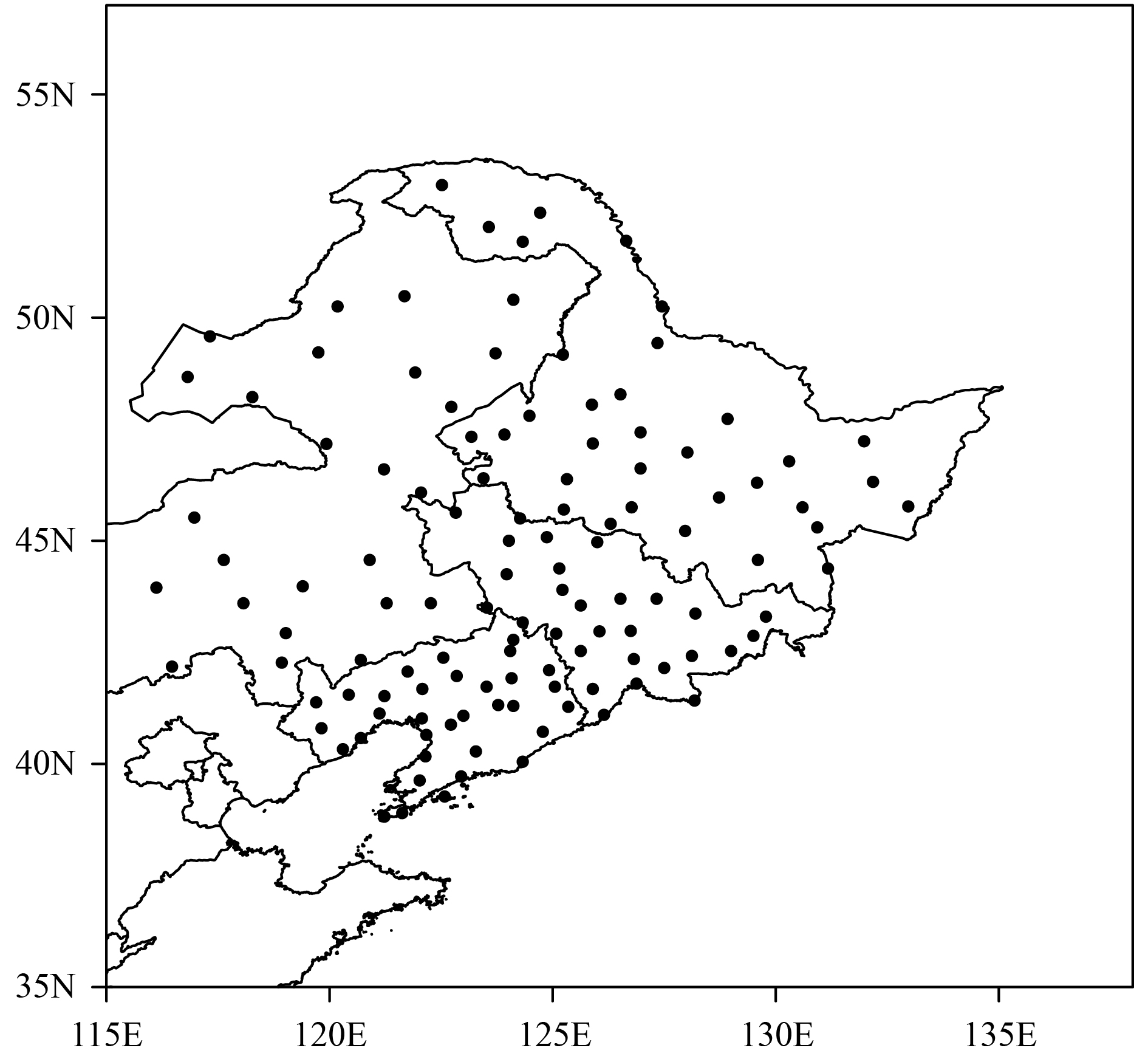
2.2 DataThe snow cover fraction datasets used for the assimilation in the present study were from the FY-3 product and are derived from different optical remote sensing platforms by using visible light, an infrared scanning radiometer, and a high-resolution spectral imager. In addition, FY-3 SD data were used to constrain the FY-3 snow cover fraction for quality control. Daily observations of the snow cover fraction from MODIS with 0.05° climate model grid (CMG) cells were used to evaluate the snow cover fraction. The study domain included 117 SD stations (Fig. 1) to evaluate the SD results produced by the Noah model during the study period (from 1 September 2011 to 1 September 2014).
|
| Figure 1 Study domain covering the Heilongjiang, Jilin, and Liaoning provinces along with the eastern Inner Mongolia Autonomous Region. Black dots represent the snow depth (SD) observation sites |
FY-3 observations of the snow cover fraction were used for the snow cover fraction assimilation in the present study. The FY-3 Multi-Sensor Synergy (MULSS) snow product fuses two results from different optical remote sensing platforms for visible light, an infrared scanning radiometer, and a high-resolution spectral imager. The FY-3 snow cover fraction data are collected globally on a daily basis. The spatial resolution of the snow cover product is 1 km; this product was mapped to 0.05° CMG cells for use in the snow cover fraction assimilation experiments in this study. Examination of the data shows that the FY-3 snow cover fraction accuracy is higher than 90% (Zhang Y. H. et al., 2015; Wu et al., 2018; Zhang et al., 2018).
2.2.2 FY-3 SD observationsFY-3 SD data were used to constrain the FY-3 snow cover fraction. The daily products include daily snow water equivalent and SD products for both the Northern and Southern Hemispheres. The microwave radiation imager’s correlated channel brightness data were used on a 25-km resolution with azimuth projections of both the Northern and Southern Hemispheres for daily readings (http://satellite.nsmc.org.cn/PortalSite/default.aspx). The FY-3 SD data algorithm is a semiempirical inversion algorithm for snow parameters in China (Jiang et al., 2014). In the research of Liu et al. (2018), the overall accuracy of the FY-3 algorithm was the highest of all the tested algorithms. The accuracy of the SD products is better than 10 cm (Wu et al., 2018).
2.3 Evaluation datasets 2.3.1 MODIS snow cover fraction productThe snow cover fraction results were evaluated against the MODIS snow cover fraction (MOD10C1) remote-sensing observations. This dataset was generated from snow cover data from the normalized difference snow index in the MOD10A1 dataset. MOD10A1 observations on a 500-m resolution were mapped to 0.05° CMG cells, binned by observation type (e.g., snow, snow-free land, and cloud), and tallied. Snow and cloud cover percentages were generated by computing the ratios of the numbers of snow or cloud observations to the total number of land observations that were mapped into each CMG cell (http://nsidc.org/data). MODIS snow products have an accuracy of approximately 90% without the effects of snow conditions or surface cover types (Hall and Riggs, 2007). Simultaneously, the quality of MODIS snow products in China has been widely verified. The accuracy of MOD10A1 in the northern part of Xinjiang, Northwest China is very high under the clear sky view; the overall accuracy of the MODIS snow cover mapping algorithm is as high as 98.5%, and the snow accuracy reaches 98.2% (Zhang et al., 2008).
2.3.2 SD station observationSD station observations for evaluating snow simulations from the land surface model were provided by the National Meteorological Information Center of China. These SD data are manually observed and reliable. A total of 117 sites with stable data quality were selected in northeastern China in the present study (Fig. 1). These stations were located in cropland (30.8%), grassland (38.4%), forest (7.7%), woodland (2.7%), shrubland (6.8%), and mixed land (13.6%). Daily SD data from these sites collected from 2011 to 2014 were used in this study. The SD data were converted from centimeter into meter during the evaluation process. The in-situ observations were preprocessed, reliable site observations were selected, and missing records were deleted.
3 Noah model, methods, and experimental design 3.1 Noah modelThe NCEP of the United States developed, optimized, and improved the Noah land surface model. The Noah model depicts the exchange of water in the snow–vegetation–soil mixing layer and simulates the snow accumulation, sublimation, melting, and associated heat transfer, in which aging, freezing, compacting, and dynamic SD, as well as density change processes, are considered. The model can output snow water equivalent (SWE), SD, and snow density and can be used to calculate snow cover fraction based on the region’s empirical ablation curve. Noah versions 3.3–3.6 adopt a snow cover fraction parameterization scheme (Koren et al., 1999) that emphasizes the relationship between the snow coverage rate and SWE. Many scholars have further studied and evaluated this model (e.g., Zhang et al., 2016). The relationships between the snow cover fraction, SWE, and SD were calculated by using Eqs. (1) and (2):
| $ {\rm{RSNOW = SNEQV/SNUP,}}\quad\quad\quad\quad\quad\quad $ | (1) |
| $ \begin{split} {\text{SNCOVR = }} & 1.0 - [{\text{exp}}(- {\rm SALP} \times {\rm RSNOW}) \\ & - {\rm RSNOW} \times {\rm exp}(- {\rm SALP})], \end{split} $ | (2) |
where SNCOVR is snow cover, SNEQV is SWE, SNUP is the SD threshold when the snow cover fraction equals 1, RSNOW is the ratio of SNEQV to SNUP, and SALP is an adjustable coefficient.
The Noah 3.6 land surface model is taken as the mo-del operator for snow cover fraction assimilation, and SD and SWE are state variables of the land surface model. EnKF is used to assimilate the FY-3 snow cover fraction products into the Noah land surface model, and the state variables of the model are updated. The snow cover ablation curve describes the relationship between snow cover and SD in Noah 3.3–3.6, and is used as an observation operator in the snow cover fraction assimilation by use of Eqs. (1) and (2).
3.2 Methods 3.2.1 EnKFIn the present study, the Noah 3.6 model was driven by CLDAS-2.0 forcing, and the EnKF (Evensen, 2003) method was used to assimilate the FY-3 snow cover fraction product. Downward shortwave radiation (SW) and precipitation (PRCP) are subject to multiplicative perturbations with a mean of 1 and standard deviations of 0.1 (SW) and 0.5 (PRCP), respectively. Zero-mean additive perturbations are applied to air temperature (T) and longwave radiation (LW) with standard deviations of 0.5 K (T) and 15 W m–2 (LW), respectively. The Noah model prognostic variables for SWE and SD are subject to multiplicative perturbations with mean = 1 and standard deviation = 0.01. A total of 25 members and the perturbation method in Table 1 were used for the EnKF runs following the methods of De Lannoy et al. (2012), with an assumption that the disturbance of these variables obeys the normal distribution. The standard deviation of the snow cover fraction in snow cover fraction assimilation was set to 0.1, which was identified according to Su et al. (2008) and Andreadis and Lettenmaier (2006).
| Variable | Perturbation method | Standard deviation | |
| Model states | SWE | Multiplicative | 0.01 (–) |
| SD | Multiplicative | 0.01 (–) | |
| Forcing | SW | Multiplicative | 0.1 (–) |
| LW | Additive | 15 W m–2 | |
| PRCP | Multiplicative | 0.5 (–) | |
| T | Additive | 0.5 K | |
| Observation | SCF | Multiplicative | 0.1 |
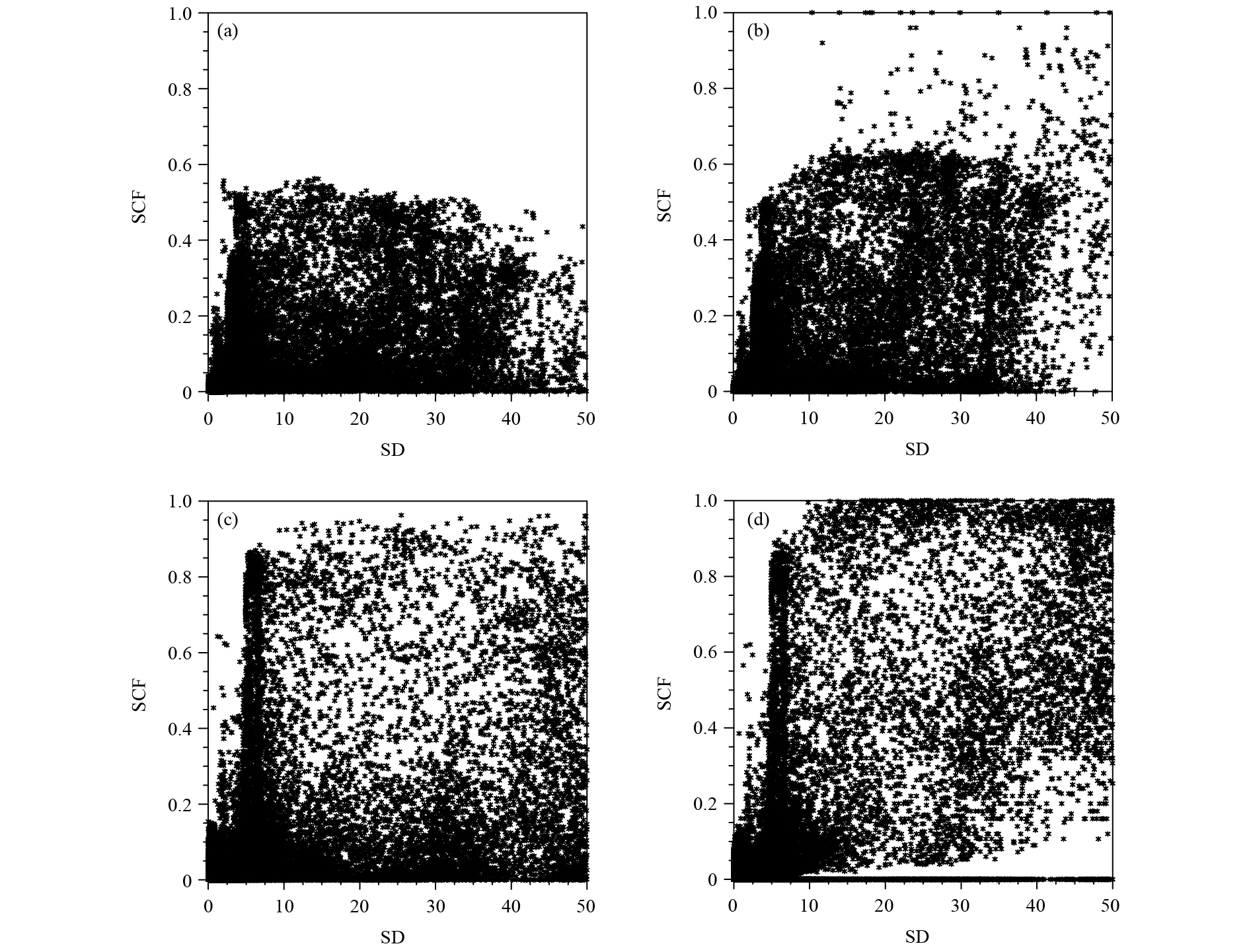
Without quality control on the snow cover products, erroneous observations may be assimilated, and erroneous results would be produced. Therefore, quality control of snow cover products is very important. The scatter plots of averaged monthly snow cover fraction and SD, based on the FY-3 0.05° daily snow cover fraction and 0.25° SD data from November 2013 to April 2014, are shown in Figs. 2a, c, which reveal some problems as follows: (1) in some grid cells, the snow cover fraction was small (nearly 0), but the SD was very large; and (2) the SD was 0 in some grid cells, but the snow cover fraction was 1.
|
| Figure 2 Scatter plots of snow cover fraction (SCF) and snow depth (SD) from the FY-3 0.05° daily SCF and 0.25° SD (cm) products (a, b) for November 2013–April 2014 and (c, d) in February 2014. (a, c) SCFDA and (b, d) SCFDA_WSD. |
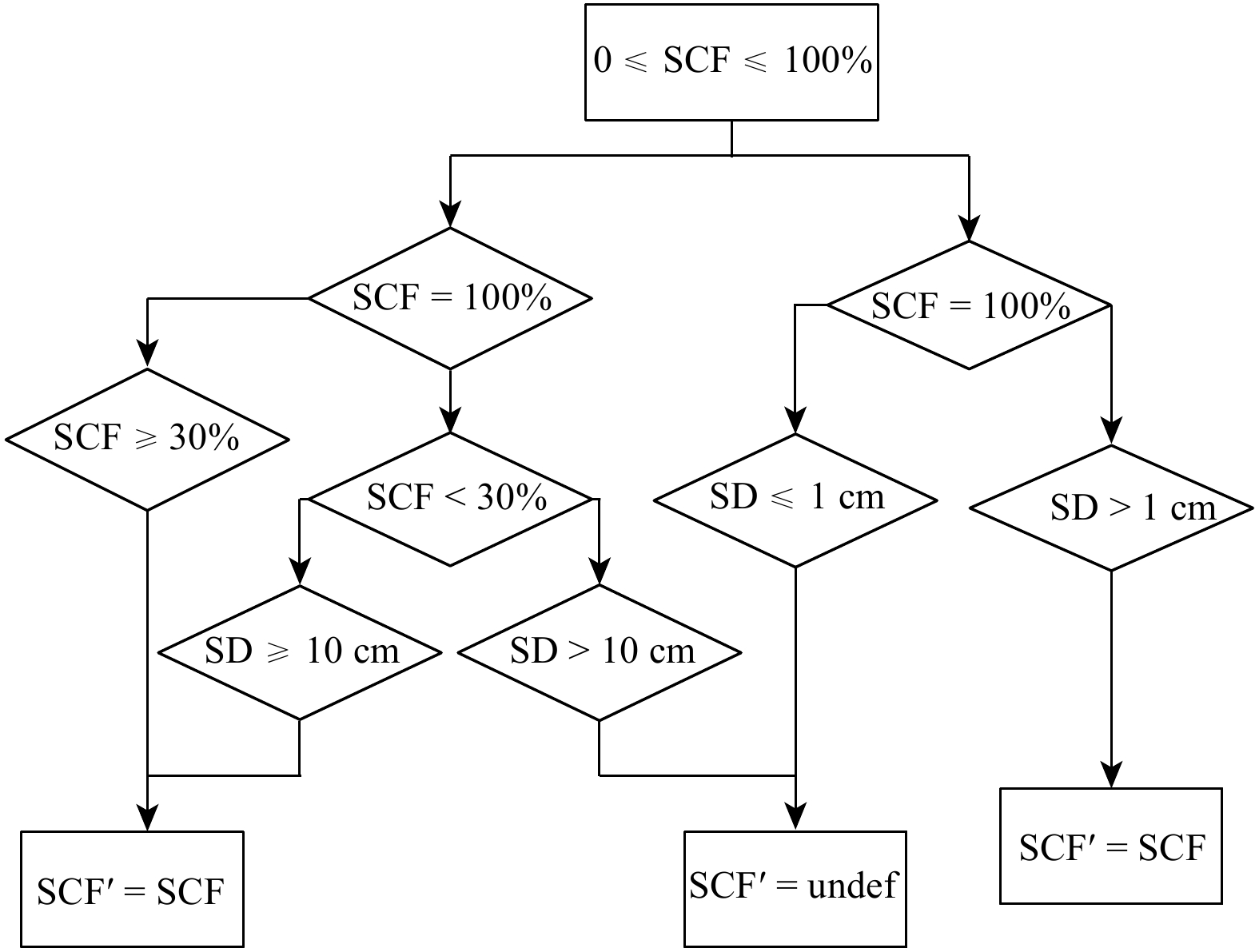
The above situations in Figs. 2a, c are unreasonable. Therefore, it is necessary to use SD data to control the quality of remote sensing snow cover products. Figure 3 is a flow chart of the process used for FY-3 snow cover fraction quality control. The following unreasonable snow cover fractions must be assigned default values (−9999.0) to avoid assimilating these unreasonable values into the model: (1) when the snow cover fraction of the grid is 100% but the SD is less than 1 cm, and (2) when the snow cover fraction of the grid is less than 30% but the SD is greater than 10 cm. In Fig. 3, SCF is the original FY-3 snow cover fraction, SCF′ is the processed (quality controlled) FY-3 snow cover fraction, SD is the FY-3 SD, and undef stands for missing value, which is set to −9999.0 in this study.
|
| Figure 3 Flow chart of FY-3 snow cover fraction (SCF) quality control. |
To illustrate the effects of the quality control on the snow cover fraction assimilation, a series of experiments were carried out by using the FY-3 snow cover fraction, which was assimilated into the Noah model. The CLDAS-V2.0 (CMA Land Data Assimilation System version 2) forcing data were obtained from the National Meteorological Information Center of China, and the Noah 3.6 model was run from arbitrary initial conditions for 21 yr by cycling the CLDAS forcing data from 1 January 2008 to 31 December 2014, with three repetitions for the spin-up. The meteorological forcing analyses with hourly products covering the region of Asia (0°–65°N, 60°–160°E) have a spatial resolution of 0.0625° × 0.0625°, and these forcing data have a good effect on snow simulation in winter (Shi et al., 2018). The Noah 3.6 land surface model was run from 1 January 2008, and began to carry out the FY-3 snow cover fraction assimilation experiments from 1 November 2011. Model runs were carried out at 6.25 km and hourly resolutions. The grid data were processed at the model resolution (0.0625°).
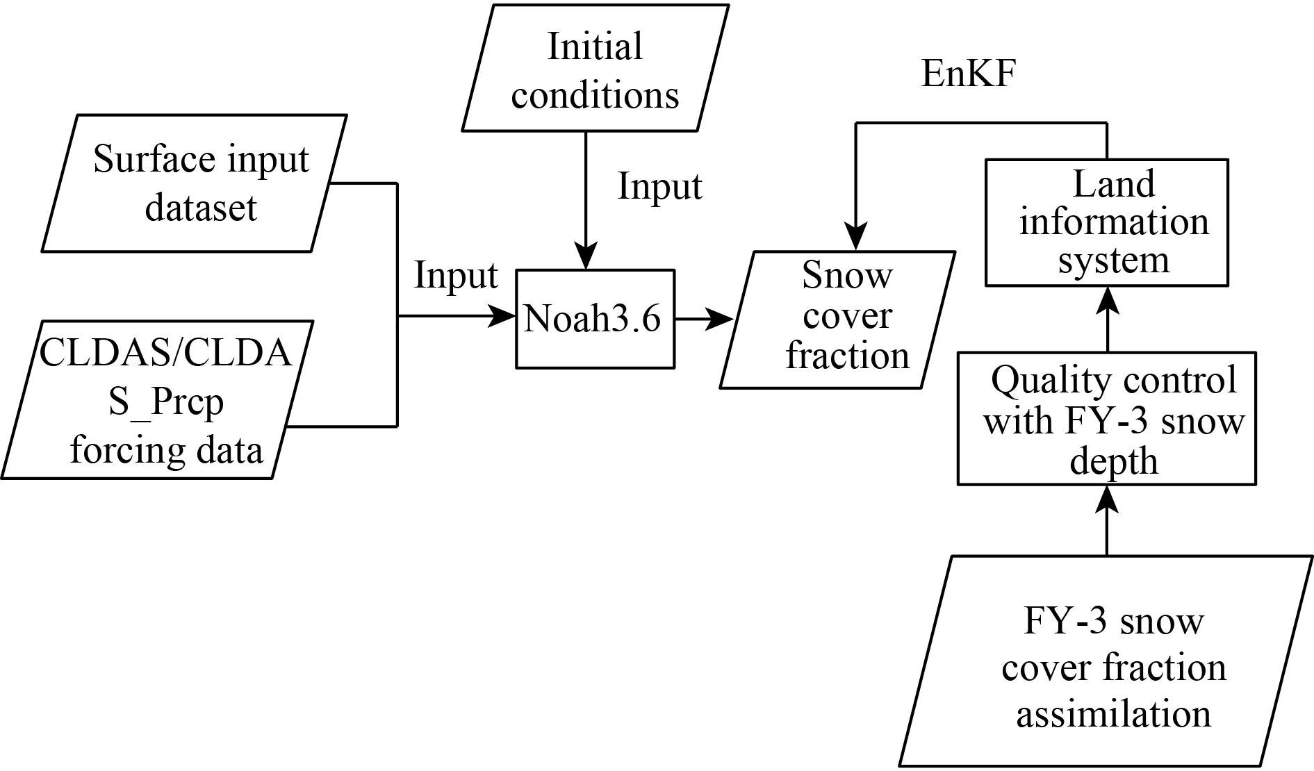
In the FY-3 snow cover assimilation experiment, the surface parameters were first input into the land surface model, and the Noah model was driven by CLDAS-2.0 forcing data to obtain stable initial conditions; then, the snow cover simulation was started. Snow cover fraction products were assimilated at a daily frequency. The snow cover fraction product was assimilated at 1330 local solar time to be close to the overpass time of FY-3B. The snow cover fraction was quality controlled from a microwave radiation imager SD product before assimilation, and then EnKF was used to assimilate snow cover products to update the SD and water equivalent in the Noah model, and the assimilation results of snow variables were then examined. Figure 4 shows a flow chart of FY-3 snow cover fraction assimilation.
|
| Figure 4 Flow chart of FY-3 snow cover fraction assimilation. |
The FY-3 snow cover fraction assimilation was carried out, and the improved effects of the assimilation were verified against the MODIS remote-sensing satellite products. The SD results were compared with the SD station observations. This paper used the BIAS, root mean square error (RMSE), and correlation coefficient (R) as evaluation indices as follows:
| $ {\rm BIAS} = {N^{ - 1}}\sum\nolimits_{i = 1}^N {\left[{{X_{\rm m}}(i) - {X_{\rm o}}(i)} \right]}, \quad\quad\; $ | (3) |
| $ {\rm RMSE} = \sqrt {{N^{ - 1}}\sum\nolimits_{i = 1}^N {{{\left[ {{X_{\rm m}}(i) - {X_{\rm o}}(i)} \right]}^2}} }, $ | (4) |
| $ \begin{aligned} & R = \\ & \frac{{\displaystyle\sum\limits_{i = 1}^N {[{X_{\rm m}}(i) - {N^{ - 1}}\displaystyle\sum\limits_{i = 1}^N {{X_{\rm m}}(i)}][{X_{\rm o}}(i) - {N^{ - 1}}\displaystyle\sum\limits_{i = 1}^N {{X_{\rm o}}(i)}]} }}{{\sqrt {\displaystyle\sum\limits_{i = 1}^N {{{[{X_{\rm m}}(i) - {N^{ - 1}}\displaystyle\sum\limits_{i = 1}^N {{X_{\rm m}}(i)}]^2}}} } \sqrt {\displaystyle\sum\limits_{i = 1}^N {{{[{X_{\rm o}}(i) - {N^{ - 1}}\displaystyle\sum\limits_{i = 1}^N {{X_{\rm o}}(i)}]^2}}} } }}, \end{aligned} $ | (5) |
where Xo represents the observation, Xm represents the model value, and N is the total number of observations.
4 Results 4.1 Quality control of snow cover productsScatter plots of monthly average snow cover fraction and snow depth are drawn based on the FY-3 0.05° daily snow cover fraction and 0.25° daily SD products from November 2013 to April 2014 (Figs. 2b, d). The number of irrational points was greatly reduced compared to that before quality control (snow cover fraction is 0, so SD is high). Before quality control, because the snow cover fraction of many points equaled 0, the monthly average snow cover fraction was small (basically below 0.5), which led to an average monthly snow cover fraction of 0 and an average monthly SD above 50 cm. After quality control, such points were reduced, with a less “thick” graphic showing reduced points of SCF = 0 and large SD; these points accounted for only 0.3% of all grid points. Because of the quality control, fewer irrational snow grids were taken into the assimilation.
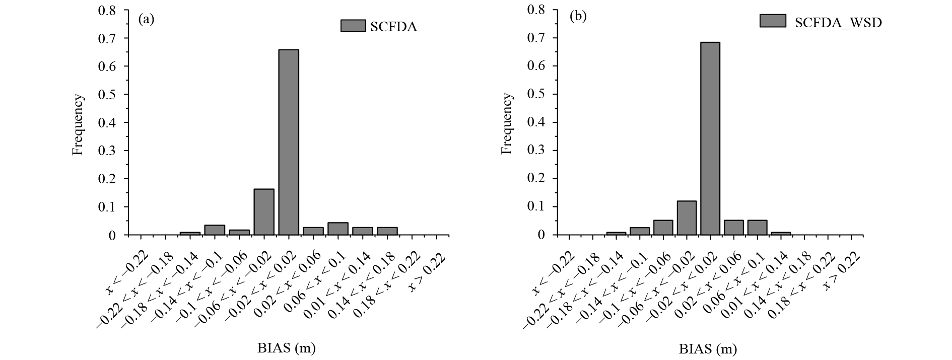
Figures 5a and 5b show the BIAS histogram of the SD from November 2013 to April 2014 before and after quality control. Clearly, the BIAS in Fig. 5a is mainly concentrated between −0.06 and 0.02 m, whereas the BIAS in Fig. 5b is mainly concentrated between −0.02 and 0.02 m; the large BIAS values are reduced, and the histogram distribution in Fig. 5b is closer to the normal distribution. It is believed that considerable erroneous snow data points with snow cover fraction of 0 and SD of large values were eliminated during the quality control process.
|
| Figure 5 BIAS histogram of SD output from November 2013 to April 2014. (a) SCFDA and (b) SCFDA_WSD. |
The FY-3 snow cover fraction assimilation results were evaluated and analyzed by using the MODIS snow cover fraction product. The FY-3 snow cover fraction assimilations with and without quality control (proposed in this paper) are denoted here as SCFDA_WSD and SCFDA, respectively.
Figure 6 shows distributions of the average snow cover fraction in northeastern China during the snow accumulation period (NDJ: November, December, and January) and the snowmelt period (FMA: February, March, and April) from November 2013 to April 2014. The MODIS snow cover fraction (Figs. 6a, d) shows that the snow cover in northeastern China was mainly concentrated in the western part of the Greater Khingan Mountains in Inner Mongolia and the eastern part of Heilongjiang Province. The snow cover fraction values were mostly within 40%–60%. It was lower in the snowmelt period than in the snow accumulation period. SCFDA_WSD inFigs. 6c, f reduces the snow cover overestimations in Heilongjiang and Jilin provinces. The magnitude and spatial distribution of SCFDA_WSD were more consistent with the observations than those of SCFDA in Figs. 6b, e.

|
| Figure 6 Distributions of the average snow cover fraction (%) during the (a, b, c) snow accumulation period (NDJ: November, December, and January) and (d, e, f) snowmelt period (FMA: February, March, and April) in northeastern China. (a, d) MODIS observations, (b, e) SCFDA, and (c, f) SCFDA_WSD. |
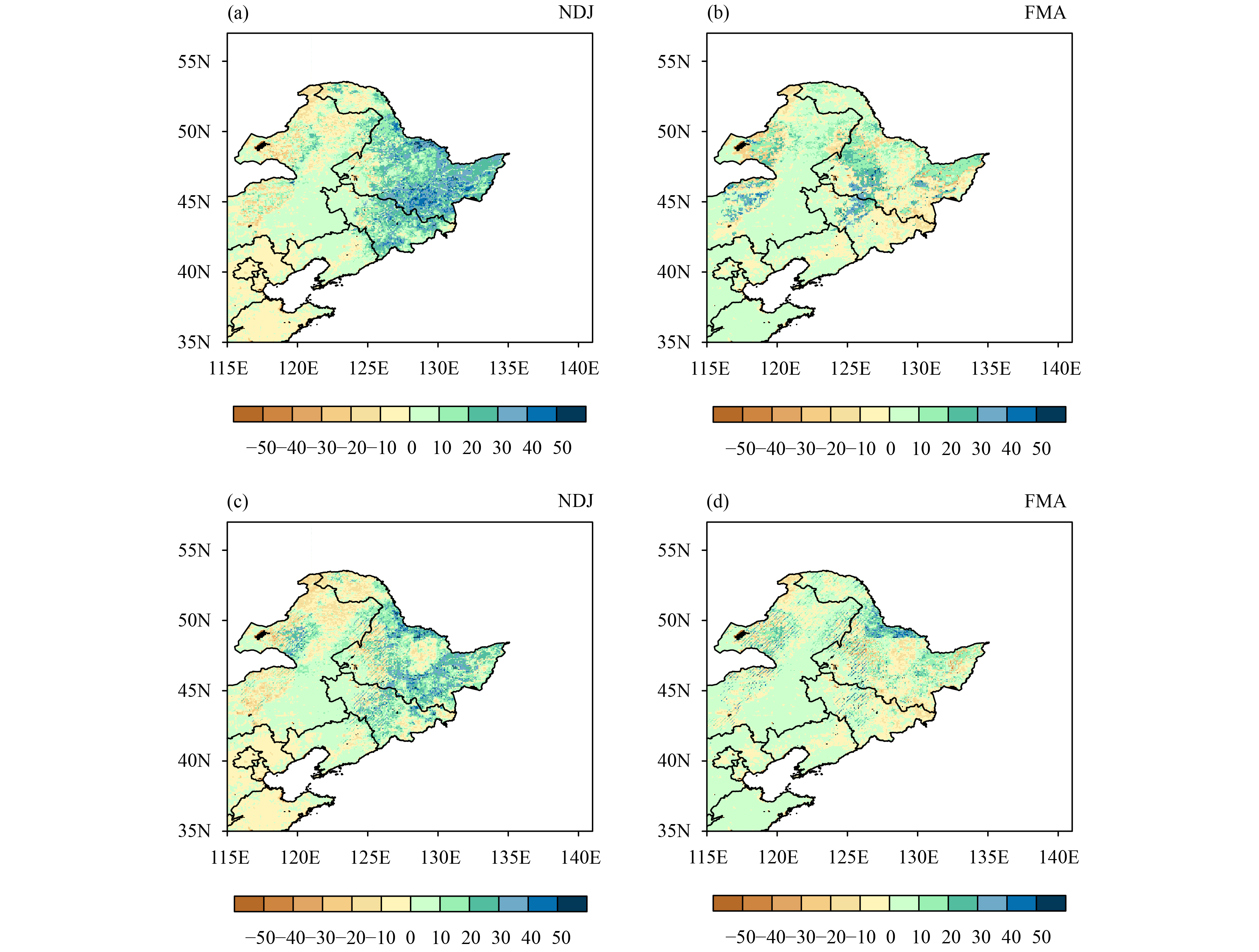
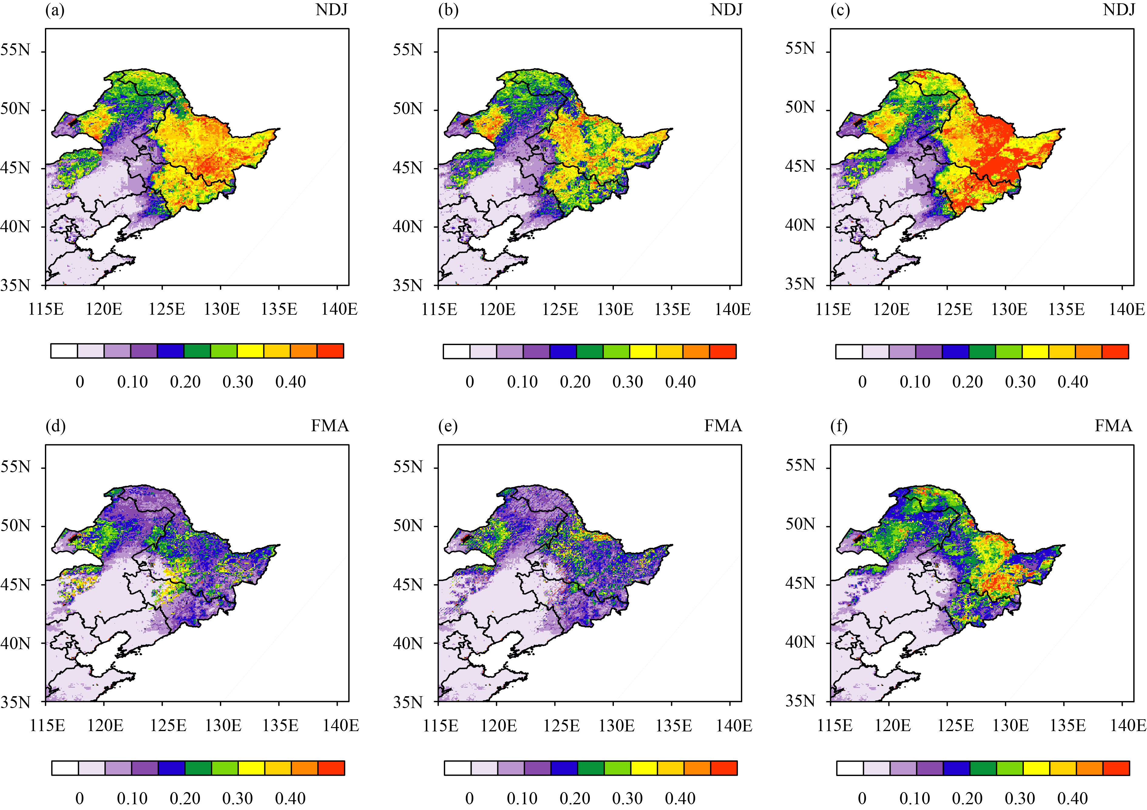
The BIAS and RMSE of the SCFDA snow cover fraction were large in northeastern China, and the improvement achieved by SCFDA in northeastern China (BIAS in Figs. 7a, b and RMSE in Figs. 8a, d) was insignificant. It is believed that erroneous snow information was assimilated, resulting in too much snow. In addition, the SCFDA_WSD result was significantly improved in northeastern China (see BIAS in Figs. 7c, d and RMSE in Figs. 8b, e), with reduced snow cover fraction in the overestimated areas and significantly decreased BIAS and RMSE. Compared with SCFDA, the BIAS of snow cover in SCFDA_WSD decreased from 0.0905 to 0.0806 (a decrease by 9.3%) and the RMSE decreased from 0.1782 to 0.1692 (a decrease of 5%). Compared with the Open Loop simulation (Figs. 8c, f), the RMSE of SCFDA_WSD decreased by 23%. When assimilating the snow cover fraction with an SD constraint (SCFDA_WSD), snow cover fraction estimates showed a substantially larger improvement than those produced by assimilating the snow cover fraction without quality control (SCFDA). The erroneous snow information in the FY-3 snow cover fraction was reduced with the FY-3 SD constraint.
|
| Figure 7 BIAS distributions of average snow cover fraction (%) during the (a, c) snow accumulation period and (b, d) snowmelt period in northeastern China. (a, b) SCFDA and (c, d) SCFDA_WSD. |
|
| Figure 8 RMSE distributions of average snow cover fraction during the (a, b, c) snow accumulation period and (d, e, f) snowmelt period in northeastern China. (a, d) SCFDA, (b, e) SCFDA_WSD, and (c, f) Open Loop (OL, simulation). |
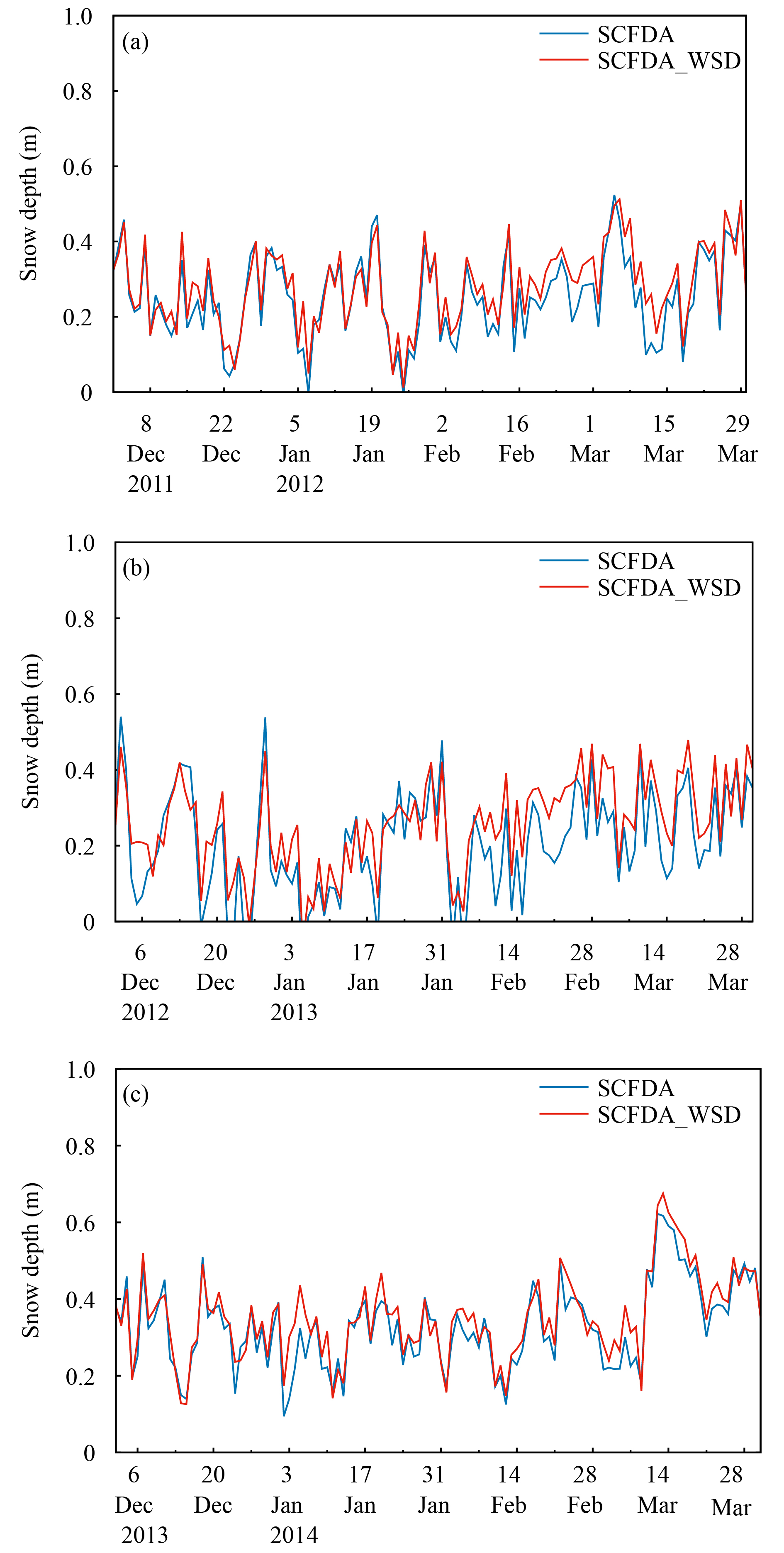
Figure 9 shows the time series of the correlation coefficient (R) in Northeast China from December to March 2011–14. Compared with SCFDA, the R values of SCFDA_WSD are significantly improved during these periods. Especially after February, the improvement in R is obvious. Figure 9 shows that SCFDA_WSD has a significantly larger improvement than SCFDA.
|
| Figure 9 Time series of the correlation coefficient in Northeast China from December 2011 to March 2014. (a) December 2011 to March 2012, (b) December 2012 to March 2013, and (c) December 2013 to March 2014 |
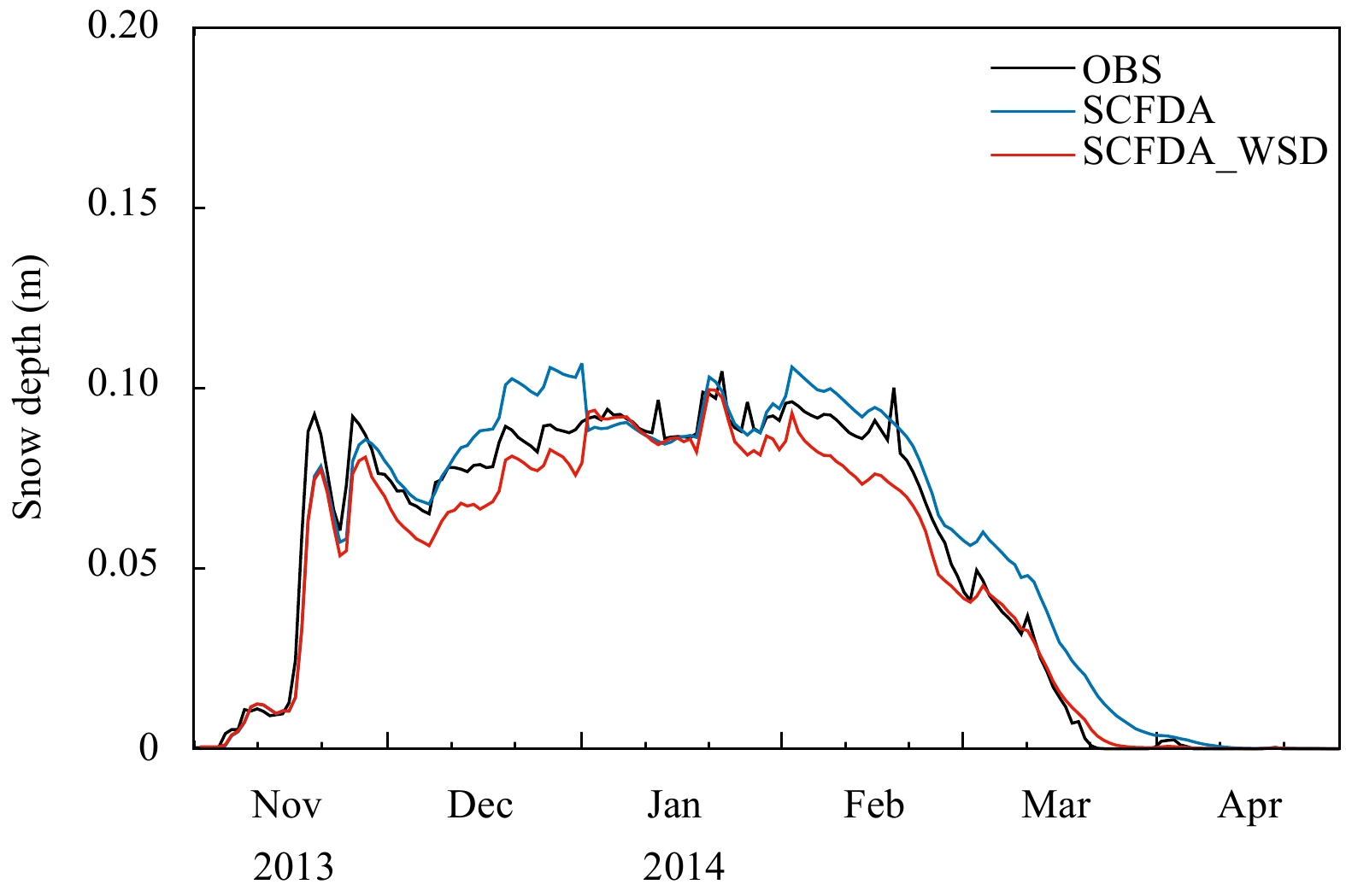
The SD simulation results were evaluated against the station SD data. Figure 10a shows the time series of the average SD of the selected in-situ SD measurements (117 points) in northeastern China from November 2013 to April 2014. In some grids, the assimilated snow cover fraction may be inconsistent with the actual fraction at some stations, resulting in an abnormal SD. The SD BIAS in SCFDA_WSD was reduced more significantly than that in SCFDA, and SCFDA_WSD successfully improved the monthly SD RMSE from 0.055 m for SCFDA to 0.043 m for SCFDA_WSD; the RMSE decreased by 21.8%, while the correlation coefficient (R) improved from 0.673 for SCFDA to 0.710 for SCFDA_WSD.
|
| Figure 10 Time series of regional mean SD in northeastern China from November 2013 to April 2014 |
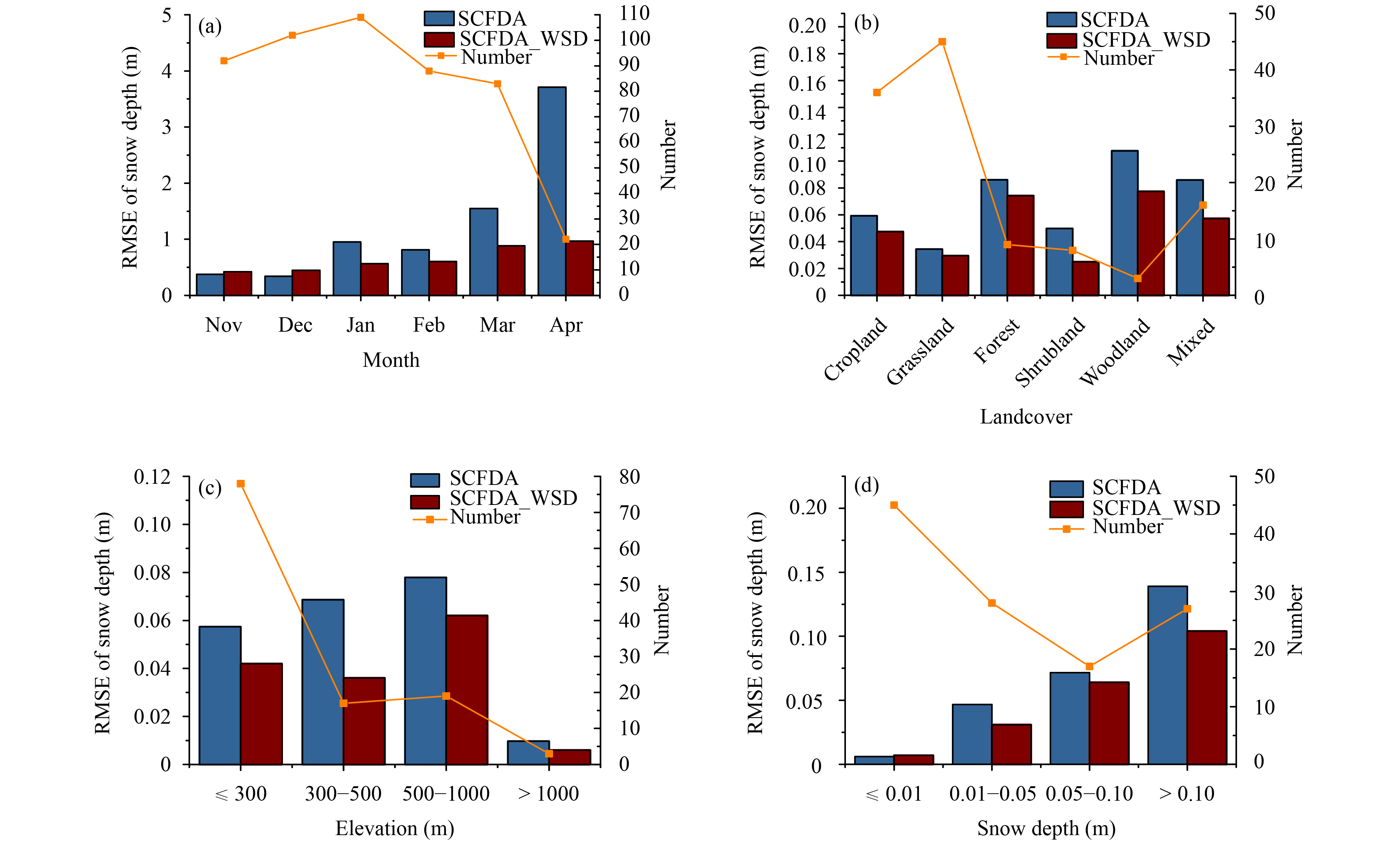
The data assimilation performance was evaluated against the SD observations for different stages, land cover types, elevations, and snow depths. The left y axis of Fig. 11 represents the RMSE, and the right y axis represents the number of stations.
|
| Figure 11 Histograms of the SD RMSE (SCFDA and SCFDA_WSD) for (a) each individual month, (b) various types of land covers, (c) various elevations, and (d) various SDs. The left y axis represents the RMSE, and the right y axis represents the number of in-situ SD measurements. |
Figure 11a shows histograms of the relative RMSE in SCFDA and SCFDA_WSD for each individual month, demonstrating that the SCFDA errors typically started small in November and gradually increased each month to a peak in April. The relative RMSE of SCFDA_WSD was relatively stable. Overall, the SCFDA_WSD achieved significant improvements over SCFDA in terms of SD values during both the snow accumulation and snowmelt periods. The reduced RMSE of the FY-3 snow cover fraction with quality control resulted in a large reduction in errors of simulated SD for all months.
The data assimilation performance was also evaluated against the SD observations for cropland, shrubland, grassland, woodland, mixed land, and forest regions. Figure 11b shows the RMSE histogram for northeastern China from November 2013 to April 2014 for different land cover types. It can be seen that the SCFDA_WSD produced an improvement in SD than the SCFDA for all land cover types. Among the various land cover types, the improvements in woodland and shrubland were the most obvious. The vegetation coverage is the main factor that influences the snow distribution, and the snow cover on woodland and shrubland is scattered. The ability of remote sensing snow products to monitor shredded snow is not sufficient; therefore, SCFDA_WSD plays an important role in areas with low vegetation cover.
Figure 11c shows a histogram of the SD RMSE for the study region from November 2013 to April 2014 for different elevations. For different altitudes, the effect of SCFDA_WSD was basically equivalent. The assimilation of SCFDA_WSD drastically reduced the SD overestimation for all elevations, and the SD RMSE was significantly reduced. The results needed to be further analyzed because samples from higher than 1000 m were limited in this study.
Figure 11d shows a histogram of the SD RMSE for northeastern China from November 2013 to April 2014 for different SD ranges. The SCFDA_WSD significantly reduced the RMSE and achieved significantly greater improvements in SD than the SCFDA for all SD ranges. The deeper the SD, the better the effect of the SCFDA_WSD.
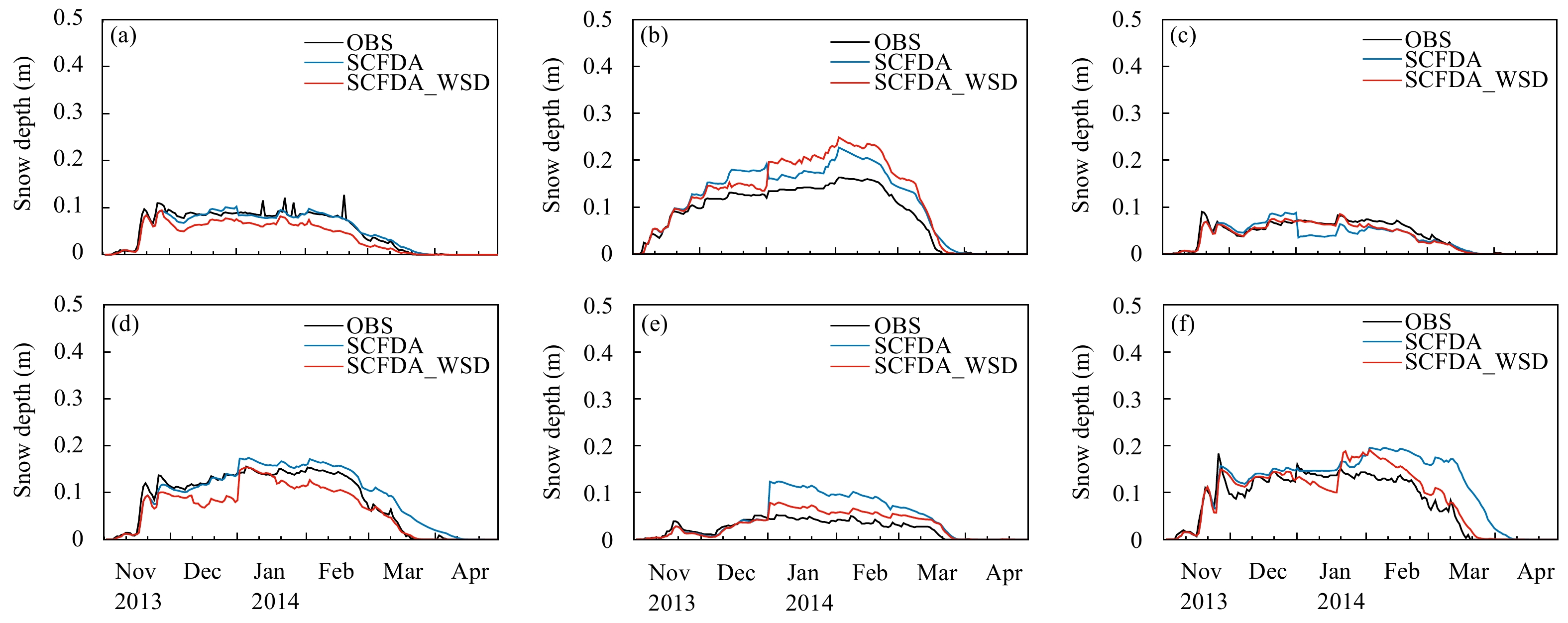
Figure 12 shows an SD time series for northeastern China from November 2013 to April 2014 for different land cover types. The data assimilation performance was significantly improved for all land cover types. The SCFDA_WSD successfully reduced the SD RMSEs of SCFDA for cropland, forests, grassland, mixed land, shrubland, and woodland (see Table 2 for specific values), respectively. In shrubland (Fig. 12e), where the SD BIAS increased early in January 2014, the SCFDA_WSD also improved, especially after January. Simultaneously, in the end of February 2014, the SD predicted by the SCFDA suddenly increased in the woodland (Fig. 12f), which should have been caused by a sudden increase in the observed snow cover fraction. These SD results were improved by the SCFDA_WSD. Of all land cover types, the improvements in SD for woodland and shrubland were the most obvious throughout the study period, and the SD results in forests were improved in the snow accumulation period.
|
| Figure 12 Time series of mean SD in northeastern China from November 2013 to April 2014 for various land cover types: (a) cropland, (b) forest, (c) grassland, (d) mixed land, (e) shrubland, and (f) woodland |
| Land cover | BIAS | RMSE | |||
| SCFDA | SCFDA_WSD | SCFDA | SCFDA_WSD | ||
| Cropland | −0.0011 | −0.0141 | 0.05924 | 0.04748 | |
| Forests | 0.0258 | 0.0318 | 0.08596 | 0.07427 | |
| Grassland | −0.0052 | −0.0034 | 0.03440 | 0.02953 | |
| Mixed | 0.0107 | −0.0162 | 0.08591 | 0.05723 | |
| Shrubland | 0.0216 | 0.0080 | 0.04979 | 0.02498 | |
| Woodland | 0.0310 | 0.0089 | 0.10760 | 0.07743 | |
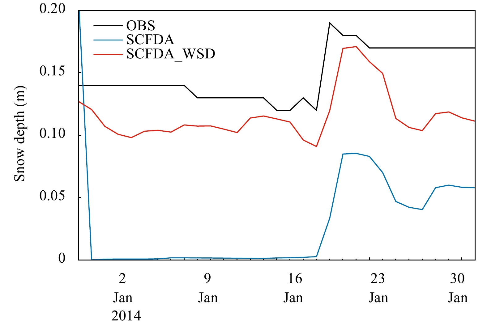
Figure 13 shows the SD time series of Huadian in Jilin Province of China during this period. The SCFDA tended to underestimate the SD, but the SCFDA_WSD effectively produced a snow accumulation curve that was in better agreement with the observations, and the SCFDA_WSD performed very well because of a reduction in the number of erroneous snow cover fraction observations. In addition, the assimilation of the FY-3 snow cover fraction with quality control resulted in a marginal improvement in the snow ablation processes. This case shows that sudden snowfall can be well reflected by the SCFDA_WSD.
|
| Figure 13 Time series of assimilated SD and observed data (m) for 19–22 January 2014 in Huadian, Jilin Province of China |
To reduce the effects of erroneous observations, which might be caused by cloud cover during the process of assimilating snow cover fraction, an improved approach was proposed in this paper: assimilation of the snow cover fraction with quality control using microwave SD products in northeastern China. The influences of quality control on the snow cover fraction assimilation were analyzed and discussed in this study.
It is concluded that considerable improvements in snow assimilation in northeastern China can be achieved by assimilating the FY-3 satellite-based snow cover fraction products with the proposed quality control. Regarding assimilation of the snow cover fraction with a snow depth constraint (i.e., quality control), the snow cover fraction and SD estimates showed substantial improvements compared to those without the quality control. The method not only performed well for all snow accumulation and snowmelt periods when compared to the observations, but also provided better agreement with the observations during a snowfall event. The SCFDA_WSD successfully reduced the SD RMSE and increased the correlation coefficient (R).
The SCFDA and SCFDA_WSD errors gradually increased each month, peaking in April, and the relative RMSE of the SCFDA_WSD remained relatively stable. Overall, the SCFDA_WSD produced improved SD estimates over the SCFDA. In addition, the data assimilation performance was evaluated against the SD observations for different stages, land cover types, elevations, and SD ranges. The SCFDA_WSD exhibited significant improvements for all land cover types. The performance improvements in woodland and shrubland were the most obvious. The SD time series for northeastern China from November 2013 to April 2014 for different land cover types showed that the SD values of grassland and shrubland were consistent with the observations, and the SD in forests was better during the snow accumulation period than during the other periods. The SD values in forest and woodland were significantly higher than the observations during the snowmelt period. For different altitudes, the effects of the SCFDA_WSD were basically equivalent. The SCFDA_WSD significantly reduced the SD RMSE and achieved significantly better results than the SCFDA for all SD ranges. The deeper the SD, the better the effect of the SCFDA_WSD.
The focus of this paper was on the assimilation of FY-3 satellite-based snow products in northeastern China. Through quality control of the observations, the influence of the observational errors was reduced during the snow cover fraction assimilation. These results reveal the importance of quality control during snow cover fraction assimilation, which is of great significance for the global use of FY-3 snow cover products. However, this paper focused on only northeastern China and assimilated only one variable—snow cover fraction. In future studies, the assimilation of SD and SWE will be performed and relevant experiments will be further conducted to improve snow and runoff predictions.
5.2 DiscussionFigure 12 shows that the SD RMSE of FY-3 snow cover assimilation with quality control (SCFDA_WSD) was less than that of SCFDA for all land cover types. The variability of each station was examined, and it was found that SCFDA_WSD was highly consistent with the observations, so the average RMSE decreased, but the improvement of the average SD was not evident in certain land cover types throughout the snowfall period. The BIAS values in cropland, forests, and mixed land from SCFDA_WSD were not significantly reduced compared to those from SCFDA. The reason might be that cropland had high vegetation coverage, and the snow cover was relatively stable. The quality of the snow cover products was high in stable snow areas, while according to the current threshold, it might have caused excessive quality control, and some real information had been lost. Figure 12b shows that the improvement effect of SCFDA_WSD was obvious at early stage of the snow accumulation period, while the BIAS increased in the late stage of the snow accumulation period. This result was possibly related to the dispersed snow cover at the early stage, but snow cover became gradually stable in the late period in the forest area, and the SCFDA_WSD played an important role in the early snow accumulation period. The effect of SCFDA_WSD on mixed land mainly depended on the proportions of the various land cover types. In addition, the SCFDA results of some cropland, forest, and mixed land sites were significantly different from the observations, although the performance of most stations had been improved. Simultaneously, optimization of the incremental formulas for state variables could be used to further improve the assimilation of snow variables in cropland, forest, and mixed land.
Acknowledgments. The snow depth dataset was provided by the National Meteorological Information Center of the China Meteorological Administration.
Appendix
The FY-3 SD data were evaluated by Ice Mapping System (IMS) snow cover observations to assess the accuracy of the data. IMS Daily Northern Hemisphere Snow and Ice Analysis provided snow and ice-cover maps from February 1997 to October 2019 by the National Snow & Ice Data Center of USA. These maps were derived from a variety of data products, including satellite imagery and in-situ data. The data were provided in ASCII text and GeoTIFF formats at three resolutions: 1, 4, and 24 km. IMS snow and ice products depict stable snow cover regions in China with good accuracy, and the annual overall accuracy rate of IMS products is greater than 92% (Liu et al., 2014). The present study used 4-km IMS snow data (
Four indices were used to evaluate the FY-3 SD data, including total accuracy (ACC), deviation (BIAS), accuracy (H), and false alarm rate (FAR). von Storch and Zwiers (2001), Stevenson (2006), and Wilks ( 2011) introduced the evaluation method. The calculations were done with Eqs. (A1)–(A4), in which a, b, c, and d are the number of pixels that are defined as: “a”: snow in both the IMS and FY-3 SD products; “b”: snow-free in the IMS product but snow in the FY-3 product; “c”: snow in the IMS product but snow-free in the FY-3 product; and “d”: snow-free in both the IMS and FY-3 products.
| $ {\rm ACC} = \frac{{a + d}}{{a + b + c + d}}, \tag{A1} $ | (A1) |
| $\hspace{-25pt} {\rm BIAS} = \frac{{a + b}}{{a + c}}, \tag{A2} $ | (A2) |
| $\hspace{-45pt} \;\; H = \frac{a}{{a + c}}, \tag{A3} $ | (A3) |
| $\hspace{-30pt} {\rm FAR} = \frac{b}{{a + b}}. \tag{A4} $ | (A4) |
ACC in Eq. (A1) represents the probability that a pixel is accurately classified, that is, the number of cells that are identical in the IMS product and the FY-3 SD product divided by the total number of pixels. However, this indicator is vulnerable to snow-free pixels and will present a value of 1 when there is no snow in summer. Therefore, an auxiliary discrimination of H is needed.
BIAS in Eq. (A2) indicates the ratio of the number of snow pixels detected by the FY-3 product to that detected by the IMS product. If the BIAS is less than 1, the number of pixels detected as snow in the FY-3 product is low. The variable H in Eq. (A3) indicates the proportion of snow pixels that account for the correct classification of the FY-3 products from all snow-covered pixels in the IMS product. FAR in Eq. (A4) represents the proportion of snow pixels that have been erroneously classified by the FY-3 product from the total number of snow cells.
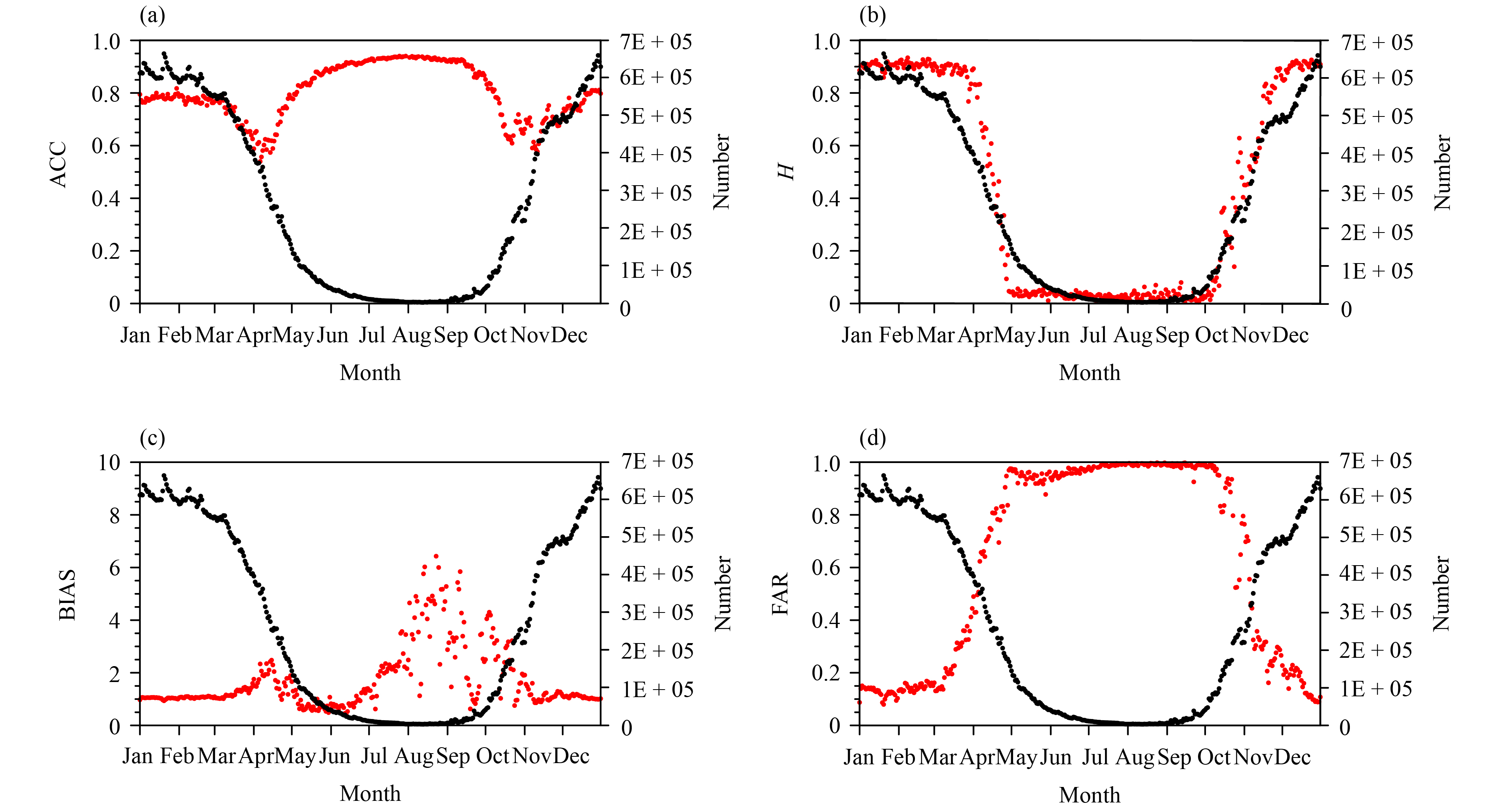
The FY-3 SD data were evaluated from 2012 to 2014 by using IMS 4-km resolution snow cover data as reference data. The IMS data are snow cover products, and different numbers indicate different land types, where 1, 2, 3, and 4 indicate water, no snow, ice, and snow, respectively. Therefore, FY-3 and IMS are considered to be the same when the following situation occurs: (1) the FY-3 SD is greater than 0 and the IMS grid value equals 4; and (2) the FY-3 SD equals 0 and the IMS grid point value is 2. Likewise, if the FY-3 SD is more than 0 and the IMS value equals 2, or if the FY-3SD is less than 0 and the IMS value is 4, the two products are considered to be different. According to the above rules, the average of the 3-yr time series from 2012 to 2014 (Fig. A1) of the ACC, BIAS,H, and FAR indicators were obtained by using Eqs. (A1)–(A4).
|
| Figure A1 Comparison between the National Snow & Ice Data Center’s Ice Mapping System (IMS) and FY-3 snow products during 2012 and 2014. (a) Total accuracy (ACC), (b) accuracy ( H), (c) deviation (BIAS), and (d) false alarm rate (FAR). The black “line” in each panel represents the number of snow pixels (corresponding to the right y axis) detected by the IMS products, while the red line represents values of each statistical index (corresponding to the left y axis) |
In Fig. A1a, the ACC value in northeastern China is consistently high, and it is generally above 0.6 and increases to between 0.8 and 0.9 during the summer, indicating that the FY-3 SD data are consistent with the IMS snow cover data. H can be used as an assessment criterion to reduce the effects of snow-free pixels in summer. The value of H varied significantly with the season, with a large value during the snow season (approximately 0.9), indicating a high degree of snow consistency in winter (Fig. A1b). During summer, H fell to 0. The BIAS in Fig. A1c reflects the ratio of the number of snow-covered pixels detected by the FY-3 SD products to the number detected by the IMS products. The BIAS was found to be nearly 1 from November to March, indicating that the number of snow pixels detected by the two products was identical. At other times, the number of snow pixels detected by FY-3 was slightly higher than that detected by IMS. FAR in Fig. A1d reflects the false-report rate of the FY-3 SD products. FAR was very low during the snow season, almost always remaining at approximately 0.1. However, in summer, the FAR values increased. Figure 12 shows that FY-3 SD data were very consistent with the IMS data during the snow season, and the quality was reliable.
| Andreadis, K. M., and D. P. Lettenmaier, 2006: Assimilating remotely sensed snow observations into a macroscale hydrology model. Adv. Water Resour., 29, 872–886. DOI:10.1016/j.advwatres.2005.08.004 |
| Bai, Y. L., X. Li, and X. J. Han, 2011: A review of error problems for land data assimilation systems. Adv. Earth Sci., 26, 795–804. DOI:10.11867/j.issn.1001-8166.2011.08.0795 |
| Che, T., 2006: Study on passive microwave remote sensing of snow and snow data assimilation method. Ph.D. dissertation, Cold and Arid Regions Environmental and Engineering Research Institute, Chinese Academy of Sciences, Lanzhou, 62 pp. (in Chinese) |
| Chen, F., 2005: Variability in global land surface energy budgets during 1987–1988 simulated by an off-line land surface model. Climate Dyn., 24, 667–684. DOI:10.1007/s00382-004-0439-4 |
| Chen, F., and J. Dudhia, 2001: Coupling an advanced land surface-hydrology model with the Penn State–NCAR MM5 modeling system. Part I: Model implementation and sensitivity. Mon. Wea. Rev., 129, 569–585. DOI:10.1175/1520-0493(2001)129<0569:CAALSH>2.0.CO;2 |
| Chen, F., K. Mitchell, J. Schaake, et al., 1996: Modeling of land surface evaporation by four schemes and comparison with FIFE observations. J. Geophys. Res. Atmos., 101, 7251–7268. DOI:10.1029/95JD02165 |
| Chen, F., Z. Janjić, and K. Mitchell, 1997: Impact of atmospheric surface-layer parameterizations in the new land-surface scheme of the NCEP mesoscale eta model. Bound.-Layer Meteor., 85, 391–421. DOI:10.1023/A:1000531001463 |
| Chen, H. S., Z. B. Sun, and W. J. Zhu, 2003: The effects of Eura-sian snow cover anomaly on winter atmospheric general circulation. Part Ⅱ: Model simulation. Chinese J. Atmos. Sci., 27, 847–860. DOI:10.3878/j.issn.1006-9895.2003.05.06 |
| Clark, M. P., A. G. Slater, A. P. Barrett, et al., 2006: Assimilation of snow covered area information into hydrologic and land-surface models. Adv. Water Resour., 29, 1209–1221. DOI:10.1016/j.advwatres.2005.10.001 |
| Crow, W. T., and R. H. Reichle, 2008: Comparison of adaptive filtering techniques for land surface data assimilation. Water Resour. Res., 44, W08423. DOI:10.1029/2008WR006883 |
| De Lannoy, G. J. M., R. H. Reichle, K. R. Arsenault, et al., 2012: Multiscale assimilation of advanced microwave scanning radiometer-EOS snow water equivalent and moderate resolution imaging spectroradiometer snow cover fraction observations in northern Colorado. Water Resour. Res., 48, W01522. DOI:10.1029/2011WR010588 |
| Dziubanski, D. J., and K. J. Franz, 2016: Assimilation of AMSR-E snow water equivalent data in a spatially-lumped snow model. J. Hydrol., 540, 26–39. DOI:10.1016/j.jhydrol.2016.05.046 |
| Evensen, G., 1994: Sequential data assimilation with a nonlinear quasi-geostrophic model using Monte Carlo methods to forecast error statistics. J. Geophys. Res. Oceans, 99, 10,143–10,162. DOI:10.1029/94JC00572 |
| Evensen, G., 2003: The ensemble Kalman filter: Theoretical formulation and practical implementation. Ocean Dyn., 53, 343–367. DOI:10.1007/s10236-003-0036-9 |
| Gao, R., H. L. Zhong, W. J. Dong, et al., 2011: Impact of snow cover and frozen soil in the Tibetan Plateau on summer precipitation in China. J. Glaciol. Geocryol., 33, 254–260. |
| Hall, D. K., and G. A. Riggs, 2007: Accuracy assessment of the MODIS snow products. Hydrol. Process., 21, 1534–1547. DOI:10.1002/hyp.6715 |
| Hall, D. K., G. A. Riggs, V. V. Salomonson, et al., 2002: MODIS snow-cover products. Remote Sens. Environ., 83, 181–194. DOI:10.1016/S0034-4257(02)00095-0 |
| Hu, Y. M., Y. H. Ding, and F. Liao, 2010: An improvement on summer regional climate simulation over East China: Importance of data assimilation of soil moisture. Chinese Sci. Bull., 55, 865–871. DOI:10.1007/s11434-009-0285-1 |
| Jiang, L. M., P. Wang, L. X. Zhang, et al., 2014: Improvement of snow depth retrieval for FY3B-MWRI in China. Sci. China Earth Sci., 44, 1278–1292. DOI:10.1007/s11430-013-4798-8 |
| Koren, V., J. Schaake, K. Mitchell, et al., 1999: A parameterization of snowpack and frozen ground intended for NCEP weather and climate models. J. Geophys. Res. Atmos., 104, 19569–19585. DOI:10.1029/1999JD900232 |
| Kumar, S. V., 2015: Assimilation of passive microwave-based soil moisture and snow depth retrievals for drought estimation. Aerosp. Sci. Technol., 45, 284–293. DOI:10.1016/j.ast.2015.05.021 |
| Kumar, S. V., C. D. Peters-Lidard, D. Mocko, et al., 2014: Assimilation of remotely sensed soil moisture and snow depth retrievals for drought estimation. J. Hydrometeor., 15, 2446–2469. DOI:10.1175/JHM-D-13-0132.1 |
| Kumar, S. V., C. D. Peters-Lidard, K. R. Arsenault, et al., 2015: Quantifying the added value of snow cover area observations in passive microwave snow depth data assimilation. J. Hydrometeor., 16, 1736–1741. DOI:10.1175/JHM-D-15-0021.1 |
| Li, H. Y., and J. Wang, 2013: Key research topics and their advances on modeling snow hydrological processes. J. Glaciol. Geocryol., 35, 430–437. DOI:10.7522/j.issn.1000-0240.2013.0051 |
| Li, P. J., and D. S. Mi, 1983: Distribution of snow cover in China. J. Glaciol. Geocryol., 5, 9–18. |
| Lin, P. R., J. F. Wei, Z.-L. Yang, et al., 2016: Snow data assimilation-constrained land initialization improves seasonal temperature prediction. Geophys. Res. Lett., 43, 11423–11432. DOI:10.1002/2016GL070966 |
| Liu, X., X. Jin, and C. Q. Ke, 2014: Accuracy evaluation of the IMS snow and ice products in stable snow covers regions in China. J. Glaciol. Geocryol., 36, 500–507. DOI:10.7522/j.issn.1000-0240.2014.0060 |
| Liu, X. J., L. M. Jiang, S. L. Wu, et al., 2018: Assessment of methods for passive microwave snow cover mapping using FY-3C/MWRI data in China. Remote Sens., 10, 524. DOI:10.3390/rs10040524 |
| Liu, Y. Q., and H. V. Gupta, 2007: Uncertainty in hydrologic modeling: Toward an integrated data assimilation framework. Water Resour. Res., 43, W07401. DOI:10.1029/2006WR005756 |
| Liu, Y. Q., C. D. Peters-Lidard, S. Kumar, et al., 2013: Assimilating satellite-based snow depth and snow cover products for improving snow predictions in Alaska. Adv. Water Resour., 54, 208–227. DOI:10.1016/j.advwatres.2013.02.005 |
| Mocko, D. M., C. D. Peters-Lidard, S. Kumar, et al., 2012: Changes to drought metrics within the North American Land Data Assimilation System (NLDAS) from the assimilation of soil moisture and snow. AGU Fall Meeting. Available at http://adsabs.harvard.edu/abs/2012AGUFM.H31L.07M. |
| Pitman, A. J., 2003: The evolution of, and revolution in, land surface schemes designed for climate models. Int. J. Climatol., 23, 479–510. DOI:10.1002/joc.893 |
| Qian, Y.-F., Y. Zhang, and Y.-Q. Zheng, 2003: Impacts of the Tibetan Plateau snow anomaly in winter and spring on precipitation in China in spring and summer. Arid Meteor., 21, 1–7. |
| Reichle, R. H., 2008: Data assimilation methods in the Earth sciences. Adv. Water Resour., 31, 1411–1418. DOI:10.1016/j.advwatres.2008.01.001 |
| Reichle, R. H., D. B. McLaughlin, and D. Entekhabi, 2002: Hydrologic data assimilation with the ensemble Kalman filter. Mon. Wea. Rev., 130, 103–114. DOI:10.1175/1520-0493(2002)130<0103:HDAWTE>2.0.CO;2 |
| Sellers, P. J., R. E. Dickinson, D. A. Randall, et al., 1997: Modeling the exchanges of energy, water, and carbon between continents and the atmosphere. Science, 275, 502–509. DOI:10.1126/science.275.5299.502 |
| Shi, C. X., S. Zhang, S. Sun, et al., 2018: Effect of improved precipitation CLDAS on snow simulation in China. Meteor. Mon., 44, 985–997. DOI:10.7519/j.issn.1000-0526.2018.08.001 |
| Stevenson, M., 2006: Book review on Ian T. Jolliffe, David B. Stephenson, Forecast Verification: A Practitioner’s Guide in Atmospheric Science, John Wiley and Sons, Chichester (2003), ISBN: 0-471-49759-2 . Int. J. Forecasting, 22, 403–405. DOI:10.1016/j.ijforecast.2005.11.002 |
| Stigter, E. E., N. Wanders, T. M. Saloranta, et al., 2017: Assimilation of snow cover and snow depth into a snow model to estimate snow water equivalent and snowmelt runoff in a Himalayan catchment. Cryosphere, 11, 1647–1664. DOI:10.5194/tc-11-1647-2017 |
| Su, H., Z. L. Yang, G.-Y. Niu, et al., 2008: Enhancing the estimation of continental-scale snow water equivalent by assimilating MODIS snow cover with the ensemble Kalman filter. J. Geophys. Res. Atmos., 113, D08120. DOI:10.1029/2007JD009232 |
| Toure, A. M., R. H. Reichle, B. A. Forman, et al., 2018: Assimilation of MODIS snow cover fraction observations into the NASA catchment land surface model. Remote Sens., 10, 316. DOI:10.3390/rs10020316 |
| von Storch, H., and F. W. Zwiers, 2001: Statistical Analysis in Climate Research. Cambridge University Press, Cambridge, 3–10. |
| Wang, H. W., C. L. Huang, J. L. Hou, et al., 2016: Estimation of snow depth from multi-source data fusion based on data assimilation algorithm. Geomatics Inf. Sci. Wuhan Univ., 41, 848–852. DOI:10.13203/j.whugis20140568 |
| Wilks, D. S., 2011: Statistical Methods in the Atmospheric Sciences. Elsevier/Academic Press, Amsterdam, 380 pp. |
| Wu., S. L., C. Liu, and J. Chen, 2018: Overview of FY-3 snow monitoring products and applications in remote sensing service. Aerosp. Shanghai, 35, 60–65. DOI:10.19328/j.cnki.1006-1630.2018.02.007 |
| Xia Y. L., Z. C. Hao, C. X. Shi, et al., 2019: Regional and global land data assimilation systems: Innovations, challenges, and prospects. J. Meteor. Res., 33, 159–189. DOI:10.1007/s13351-019-8172-4 |
| Xiao, L., and T. Che, 2015: Preliminary study on snow feedback to the climate system in the Tibetan Plateau. Remote Sens. Technol. Appl., 30, 1066–1075. DOI:10.11873/j.issn.1004-0323.2015.6.1066 |
| Xu, J. H., and H. Shu, 2016: DEnKF-based assimilation of MODIS-derived snow cover products into common land model considering the model sub-grid heterogeneity. Geomatics Inf. Sci. Wuhan Univ., 41, 156–162. DOI:10.13203/j.whugis20140039 |
| Xu, L. Y., and B. Y. Wu, 2012a: Two physical effects of Eurasian snow cover on the late-spring and early-summer rainfall in South China of 2010. Chinese J. Atmos. Sci., 36, 271–282. DOI:10.3878/j.issn.1006-9895.2011.11054 |
| Xu, L. Y., and B. Y. Wu, 2012b: Relationship between Eurasian snow cover and late-spring and early-summer rainfall in China in 2010. Plateau Meteor., 31, 706–714. |
| Yang, F., H. Lu., K. Yang., et al., 2017: Evaluation of multiple forcing data sets for precipitation and shortwave radiation over major land areas of China. Hydrol. Earth Syst. Sci., 21, 5805–5821. DOI:10.5194/hess-21-5805-2017 |
| Yang, K., T. T. Hu, and C. H. Wang, 2017: A numerical study on the relationship between the spring–winter snow cover anomalies over the northern and southern Tibetan Plateau and summer precipitation in East China. Chinese J. Atmos. Sci., 41, 345–356. DOI:10.3878/j.issn.1006-9895.1604.16119 |
| Yang, Z.-L., 2004: Modeling land surface processes in short-term weather and climate studies. Observation, Theory and Modeling of Atmospheric Variability, X. Zhu, X. F. Li, M. Cai, et al., Eds., Singapore, World Scientific, 288–313, doi: 10.1142/9789812791139_0014. |
| Yatheendradas, S., C. D. Peters Lidard, V. Koren, et al., 2012: Distributed assimilation of satellite-based snow extent for improving simulated streamflow in mountainous, dense forests: An example over the DMIP2 western basins. Water Resour. Res., 48, W09557. DOI:10.1029/2011WR011347 |
| Zhang, R. H., R. N. Zhang, and Z. Y. Zuo, 2016: An overview of wintertime snow cover characteristics over China and the impact of Eurasian snow cover on Chinese climate. J. Appl. Meteor. Sci., 27, 513–526. DOI:10.11898/1001-7313.20160501 |
| Zhang, R. N., R. H. Zhang, and Z. Y. Zuo, 2015: Winter snow cover variability over China and its relation to Arctic Oscillation. Chinese J. Atmos. Sci., 39, 634–642. DOI:10.3878/j.issn.1006-9895.1405.14170 |
| Zhang, S., C. X. Shi, X. Liang, et al., 2018: Assessment of FY-3 snow cover product. Remote Sens. Technol. Appl., 33, 35–46. DOI:10.11873/j.issn.1004-0323.2018.1.0035 |
| Zhang, X.-T., X.-D. Huang, T.-G. Liang, et al., 2008: Accuracy analysis for MODIS snow data of MOD10A1 in a pastoral area in northern Xinjiang. Acta Pratacult. Sinica, 17, 110–117. DOI:10.3321/j.issn:1004-5759.2008.02.016 |
| Zhang, Y.-F., T. J. Hoar, Z.-L. Yang, et al., 2014: Assimilation of MODIS snow cover through the data assimilation research testbed and the community land model version 4. J. Geophys. Res. Atmos., 119, 7091–7103. DOI:10.1002/2013JD021329 |
| Zhang, Y. H., W. Ren, T. Cao, et al., 2015: Method of snow multi-threshold comprehensive discrimination with FY-3/VIRR data. Remote Sens. Technol. Appl., 30, 1076–1084. DOI:10.11873/j.issn.1004-0323.2015.6.1076 |
| Zuo, Z. Y., and R. H. Zhang, 2012: The anomalies of spring rainfall in China and its relation with tropical pacific SST and Eurasian snow. Chinese J. Atmos. Sci., 36, 185–194. DOI:10.3878/j.issn.1006-9895.2012.01.14 |
 2019, Vol. 33


