The Chinese Meteorological Society
Article Information
- FU, Xiaolei, Zhongbo YU, Ying TANG, et al., 2019.
- Evaluating Soil Moisture Predictions Based on Ensemble Kalman Filter and SiB2 Model. 2019.
- J. Meteor. Res., 33(2): 190-205
- http://dx.doi.org/10.1007/s13351-019-8138-6
Article History
- Received August 28, 2018
- in final form December 15, 2018
2. College of Civil Engineering, Fuzhou University, Fuzhou 350116, China;
3. State Key Laboratory of Hydrology–Water Resources and Hydraulic Engineering, Hohai University, Nanjing 210098, China;
4. Department of Geography, Michigan State University, East Lansing, MI 48824, USA;
5. College of Earth and Environmental Sciences, Lanzhou University, Lanzhou 730000, China
Soil moisture content is important to various studies in hydrological, meteorological, and agricultural fields (Heathman et al., 2003; Lyu et al., 2011a; Fu et al., 2014). It influences the partitioning of rainfall into runoff or infiltration in hydrology (Western and Blöschl, 1999; Koster et al., 2004), and affects the redistribution of energy to sensible or latent heat exchange at the earth’s surface in meteorology (Koster et al., 2004). Moreover, the accurate soil moisture content estimation is essential in developing appropriate irrigation scheduling and water resource management, and in improving drought forecasting and crop production in agriculture (Milly et al., 2008; Liu D. et al., 2016). However, it is difficult to obtain long-period large-scale soil moisture observations with multiple soil depths through in-situ measurements (Li et al., 2010; Lyu et al., 2011a, b).
Over the past decades, many researchers have focused on obtaining long-term local or large-scale multi-depth soil moisture data by using the land surface model (Sellers et al., 1996; Dai et al., 2003; Oleson et al., 2004), or the hydrological model (Famiglietti and Wood, 1994; Liang et al., 1994; Xiang et al., 2016), or by remote sensing (Shi et al., 2006; Balsamo et al., 2007; Wang et al., 2016). For example, Sellers et al. (1996) developed the Simple Biosphere Model (SiB2) to obtain the soil moisture at different soil depths. The Community Land Mo-del (CLM) has been used to obtain the large-scale soil moisture data globally (Decker and Zeng, 2009; Lai et al., 2014; Luo et al., 2017). The TOPMODEL-based Land Surface–Atmosphere Transfer Scheme (TOPLATS;Famiglietti and Wood, 1994; Fu et al., 2018a) has been used to simulate the root zone soil moisture content at different spatial scales. A remote sensing technique has been used to obtain the large-scale soil moisture estimation, but it is only effective for retrieving the moisture content at the soil surface (Jackson et al., 1999, Yu et al., 2001; Balsamo et al., 2007; Wang et al., 2016). Despite of these efforts, the accuracy of the simulated or retrieved soil moisture is not sufficient as there are uncertainties associated with the models, precipitation, and input parameters in land surface or hydrological models (Dumedah and Walker, 2014), and the resolution of the surface soil moisture obtained by remote sensing is coarse.
Data assimilation is an efficient way to improve the simulation accuracy, which has been employed in soil moisture studies for several decades (Kalman, 1960; Yeh et al., 1984; Han and Li, 2008; Fu et al., 2014; Yu et al., 2014a, b; Dumedah and Walker, 2017). For example, Yeh et al. (1984) investigated the influence of short-term climate and hydrological changes on the soil moisture using the Extended Kalman Filter (EKF). Huang et al. (2008) improved the in-situ soil moisture simulation accuracy by assimilating the Tropical Rainfall Measuring Mission (TRMM) Microwave Imager (TMI) brightness temperature using the Ensemble Kalman Filter (EnKF). Han et al. (2014) used the Local Ensemble Transform Kalman Filter (LETKF) to improve the soil moisture characterization based on optimized soil properties. Lievens et al. (2016) assimilated the soil moisture and brightness temperature products of Soil Moisture and Ocean Salinity (SMOS) into the Variable Infiltration Capacity (VIC) model using the EnKF and obtained improved soil moisture results. Moreover, several existing soil moisture assimilation datasets are now available such as the global, North America, and West China soil moisture data that can be obtained from the Global Land Data Assimilation System (GLDAS; Rodell et al., 2004), North American Land Data Assimilation System (NLDAS; Luo et al., 2003; Schaake et al., 2004), and West China Land Data Assimilation System (WCLDAS; Huang and Li, 2004).
Since data assimilation can improve the soil moisture simulation results as shown by several studies, it would be of interest to understand how the assimilated results (initial values) with different assimilation frequencies before the current time influence soil moisture predictions in the future. In addition, it is important to assess the impact of precipitation on the soil moisture content. The above concerns are addressed in this study using an experiment of the soil moisture assimilation/prediction based on the SiB2 model and EnKF that was conducted at the Meilin watershed, eastern China. A description of the study area is presented in Section 2. The experiment design, descriptions of the SiB2 model and EnKF, and evaluation criteria are discussed in Section 3. Section 4 presents the results and discussion, followed by conclusions in Section 5.
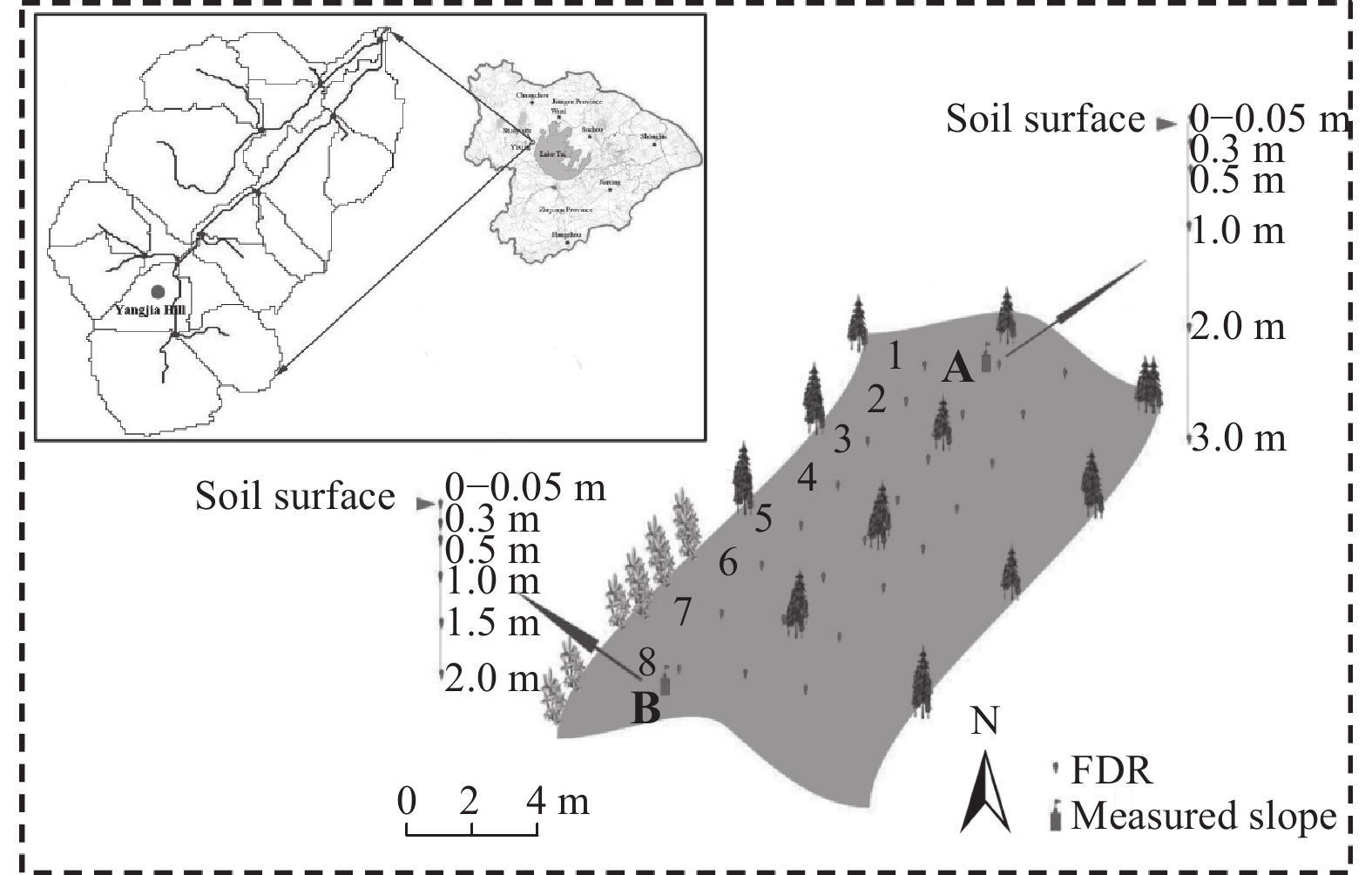
2 Meilin watershedThe Meilin watershed has a catchment area of 0.7 km2, and is located in the southeast of Yixing City, Jiangsu, China (Fig. 1). The average annual precipitation is approximately 1150 mm, and the annual average air temperature is approximately 15.5°C. Vegetation mainly includes woods (trees and bushes) and grass, and loam is the main soil type. The slope of the watershed is about 19°, and its elevation is from 15.5 to 23.8 m. In the watershed, an automatic weather station (WS-STD1) was used to record the meteorological data (e.g., relative humidity and air temperature), as well as a rain gauge to record precipitation. Two Frequency Domain Reflectometry (FDR) sensors were placed as shown in Fig. 1 at Points A and B at Yangjia Hill to automatically record the soil moisture at different soil layers. In this study, the hourly soil moisture observations from 11 August to 14 September 2007 (days 223–257) were collected at depths of 5, 50, and 100 cm at Point A (top of the watershed). Also, the hourly soil moisture observations from 1 December 2008 to 14 February 2009 (days 335–410) at Point B (bottom of the watershed) with depths of 5, 30, and 100 cm were collected. Meteorological data from 22 June to 14 September 2007 and from 14 September 2008 to 14 February 2009, were collected to investigate the influence of the initial state value and precipitation on soil moisture predictions.
|
| Figure 1 The Meilin watershed and location of soil moisture observation sites. Points A and B are focused in this study. |
This study provides an assessment of the soil moisture predictions based on SiB2 and EnKF utilizing the hourly in-situ soil moisture observations from 11 August to 14 September 2007 (days 223–257) at Point A and from 1 December 2008 to 14 February 2009 (days 335–410) at Point B. Considering the short temporal coverage of the experiment and the observations, the meteorological data (from 22 June to 10 August 2007 and from 14 September to 30 November 2008) were used to spin-up the model for 10 times at Points A and B, respectively, before undertaking the assimilation. The daily observed precipitation of the corresponding assimilation and prediction period is shown in Fig. 2, and averagely interpolated into each model running time. Once the observations are obtained, the observations can be assimilated into the model by EnKF to improve the soil moisture simulations, so the assimilation procedure can be conducted according to Fig. 3. The simulated, assimilated, and predicted soil moistures were assessed at the soil depths of 5, 50, and 100 cm at Point A, and 5, 30, and 100 cm at Point B.

|
| Figure 2 Precipitation at Points A and B in Meilin watershed, eastern China: (a) 11 August to 14 September 2007 (days 223–257) at Point A and (b) 1 December 2008 to 14 February 2009 (days 335–410) at Point B. |

|
| Figure 3 Simple scheme of the assimilation/prediction procedure. |
The time interval ∆t of the soil moisture simulation is set to be 1 h, the assimilation frequencies are set to be every one hour (hourly), every three hours, and once a day (daily). During the prediction period, the model runs without assimilation, which is shown in Fig. 3. Thus, the assimilated soil moisture, with different assimilation frequencies, at the end of assimilation period is set to be the initial state value for the soil moisture prediction period. Additionally, the precipitation in the prediction period uses the measured precipitation, the randomly generated precipitation [i.e., measured precipitation value multiplied by a random value generated from the uniform distribution U (0, 2)], and zero precipitation. There are sparse in situ soil moisture observations, and remote soil moisture is limited to the soil surface, so setting the observed soil moisture to be the initial values is only used to test whether the model is stable at the beginning of prediction period. Based on the initial value and precipitation data, six cases for Point A are considered as listed in Table 1, and only four cases for Point B are considered as listed in Table 2.
| Case | Initial value for prediction period | Precipitation in prediction period | Assimilation frequency (h) | Soil moisture result |
| 0 | Measured value | Measured value | Fig. 4 | |
| 1 | Assimilated_1h | Measured value | 1 | Figs. 5, 8 |
| 2 | Assimilated_3h | Measured value | 3 | Fig. 9 |
| 3 | Assimilated_1d | Measured value | 24 | Fig. 10 |
| 4 | Assimilated_1h | Measured × U (0, 2) | 1 | Fig. 12 |
| 5 | Assimilated_1h | 0 | 1 | Fig. 13 |
| Note: Assimilated_1h, Assimilated_3h, and Assimilated_1d represent cases with an assimilation frequency of 1 h (hourly), 3 h, and 1 day (daily), respectively. Case 0 is used to test the model stability in the prediction period. | ||||
In this study, the SiB2 model (Sellers et al., 1996) is adopted as the model operator, which can simulate the water–energy transfer process in land–atmosphere interaction. To simulate the soil moisture, three soil layers in the soil column are considered, which are the soil surface, root zone, and deep soil layers. The node for soil surface, root zone, and deep soil layers are set to be 5, 50 or 30, and 100 cm, respectively, as the soil moisture observation collected at the corresponding depths. The governing equation in each soil layer is as follows:
| $ {\rm Soil \; surface \; layer: }\;\; \frac{{\partial {W_1}}}{{\partial t}} = \frac{1}{{{\theta _{\rm{s}}}{D_1}}}\left[ {P - {Q_{1, 2}} - \frac{1}{\rho }{E_{\rm{g}}}} \right]; \;$ | (1) |
| ${\rm Root \; zone \; layer:}\;\;\frac{{\partial {W_2}}}{{\partial t}} = \frac{1}{{{\theta _{\rm{s}}}{D_2}}}\left[ {{Q_{1, 2}} - {Q_{2, 3}} - \frac{1}{\rho }{E_{\rm{c}}}} \right];$ | (2) |
| $\!\!\!\!\!\!\!\!\!\!\!\!\!\!\!\!\!\!\!\!\!\!\!\!\!\!\!\!\!\!\!\!\!\!\!\!\!\!\!\!\!\!\!{\rm Deep \; soil \; layer:}\;\;\frac{{\partial {W_3}}}{{\partial t}} = \frac{1}{{{\theta _{\rm{s}}}{D_3}}}\left[ {{Q_{2, 3}} - {Q_3}} \right]. $ | (3) |
Here, W1, W2, and W3 are the soil moisture wetness (state variables) at each soil layer (m3 m–3); θs is the saturated soil water content (m3 m–3); Di (i = 1, 2, 3) is the ith soil layer thickness (m); Qi,i+1 (i = 1, 2) is the water flow between layers i and i + 1 (m s–1); Q3 is the gravitational drainage from the recharge soil moisture store (m s–1); P is the precipitation infiltration into the soil surface layer (m s–1); Eg is the evaporation rate from the soil surface layer (m s–1); Ec is the canopy transpiration rate (m s–1); and ρ is the water density.
In this land surface model, the input variables include the precipitation, air temperature, relative humidity, wind speed, shortwave radiation, and longwave radiation. The longwave radiation is calculated by using a standard method, i.e., Brunt’s equation (Monteith, 1973), in SiB2.
3.2 Ensemble Kalman FilterThe EnKF (Evensen, 1994; Heemink et al., 2001; Vrugt et al., 2006; Weerts and Serafy, 2006; Xie and Zhang, 2010; Dumedah and Coulibaly, 2013; Liu H. R. et al., 2016; Fu et al., 2018b) has achieved a great success and is frequently applied to improve the simulation accuracy in the fields of atmosphere, hydrology, and ocean science (Whitaker and Hamill, 2002). The EnKF includes a state function M and an observation function H. M is the aforementioned SiB2 model for simulating soil moisture at different soil layers, and H is used to link the soil moisture simulations to observations in this study as follows:
| ${ X_k} = { M}\left({{{ X}_{k - 1}}, {{ V}_{k - 1}}} \right), $ | (4) |
| ${{ Y}_k} = { H}\left({{{ X}_k}, {{ U}_k}} \right), \quad\quad$ | (5) |
where Xk is the simulated value of the state variable at time k, and Xk = [W1, W2, W3]
(1) Forecasting: The initial ensembles
| ${{ X}_{k, i}} = { M}\left({{{ X}_{k - 1, i}}, {{ V}_{k - 1, i}}} \right)\;\;\;\;{{ V}_{k, i}} \sim N\left({0, { Q}} \right), $ | (6) |
where Xk,i is the forecasted soil moisture for each member at time k; N is the ensemble size, and is set to 80 in this study, as Moradkhani et al. (2005) and Vrugt et al. (2006) pointed out that the assimilated results tend to be stable when the ensemble size is larger than 50.
(2) Updating: For updating the state variable (soil moisture), the observed soil moisture is assimilated into the model by using the following equation:
| ${ X}_{k, i}^{\rm up} = {{ X}_{k, i}} + {{ K}_k}\left[ {{{ Y}_{k, i}} - {{H}}\left({ {{\bar{ X}}_k} } \right)} \right].$ | (7) |
The Kalman gain Kk and generated measurements ensemble Yk,i at time k (Weerts and Serafy, 2006) are obtained based on the following equations:
| $\!\!\!\!\!\!\!\!\!\!\!\!\!\!\!\!\!\!\!\!\!\!\!\!\!\!\!\!\!\!\!{{ K}_k} = {{ P}_k}{{ H}^{\rm T}}{\left({{ H}{{ P}_k}{{ H}^{\rm T}} + { R}} \right)^{ - 1}}, $ | (8) |
| $\!{{ Y}_{k, i}} = { H}\left({{{ X}_{k, i}}, {{ U}_{k, i}}} \right)\;\;\;\;\;{{ U}_{k, i}} \sim N\left({0, { R}} \right), $ | (9) |
| $\!\!\!\!\!\!\!\!\!\!\!\!\!\!\!\!\!\!\!\!\!\!\!\!\!\!\!\!\!\!\!\!{{H}}\left({{{\bar{ X}}_k} } \right) = \frac{1}{N}\mathop \sum \nolimits_{i = 1}^N { H} \left({{{ X}_{k, i}}} \right), \;$ | (10) |
where R is the measurement noise variance, which is set to be the unit matrix multiplied by 0.005, and Q is set to equal to R.
To obtain the Kalman gain, the error covariance matrix Pk can be calculated as follow:
| ${{ P}_k} = \frac{1}{{N - 1}}{{ E}_k}{ E}_k^{\rm T}.$ | (11) |
The error expectation in each ensemble member is obtained as follows:
| ${{ E}_k} = \left[ {{{{ X}}_{k, 1}} - {{{\bar{ X}}_k}}, \cdots, {{{ X}}_{k, N}} - {{{{\bar{ X}}}_k}} } \right], $ | (12) |
| $ {{{\bar { X}}_k}} = \frac{1}{N}\mathop \sum \nolimits_{i = 1}^N {{ X}_{k, i}}. \;\quad\quad\quad\quad\quad\quad$ | (13) |
Finally, the updated state variable value at time k can be obtained as follow:
| ${ X}_k^{\rm up} = \frac{1}{N}\mathop \sum \nolimits_{i = 1}^N { X}_{k, i}^{\rm up}.$ | (14) |
When the measurements are a nonlinear combination of state variables, PHT and HPHT can be directly calculated by using the following equations (Houtekamer and Mitchell, 2001; Huang et al., 2008):
| $\!\;\;{{P}}{{{ H}}^{\rm T}} = \frac{1}{{N - 1}}\mathop \sum \nolimits_{i = 1}^N \left[ {{{ X}_{k, i}} - { {\bar X}}} \right]{\left[ {{ H} \left({{{ X}_{k, i}}} \right) - { H}\left({ {\bar X}}\right)} \right]^{\rm T}}, $ | (15) |
| ${{HP}}{{{H}}^{\rm T}} = \frac{1}{{N - 1}}\mathop \sum \nolimits_{i = 1}^N \left[ {{ H}\left({{{ X}_{k, i}}} \right) - { H} \left({ {\bar X} }\right)} \right]{\left[ {{ H}\left({{{ X}_{k, i}}} \right) - { H}\left({ {\bar X}} \right)} \right]^{\rm T}}.$ | (16) |
To analyze how the initial state value and precipitation affect the soil moisture prediction, the Root-Mean-Square Error (RMSE), Absolute Error (AE), and daily average bias (Bias) are used and calculated as follows:
| ${\rm{RMSE}} = \sqrt {\frac{1}{n}\mathop \sum \nolimits_{k = 1}^N {{\left({{{ X}_{{\rm{pred}}, k}} - {{ X}_{{\rm{obs}}, k}}} \right)}^2}}, $ | (17) |
| $\!\!\!\!\!\!\!\!\!\!\!\!\!\!\!\!\!\!\!\!\!\!{\rm{AE}} = \left| {{{ X}_{{\rm{pred}}, k}} - {{ X}_{{\rm{obs}}, k}}} \right|, \quad\quad\quad\quad$ | (18) |
| $\!\!\!\!\!\!\!\!\!\!\!\!\!\!\!\!\!\!\!\!\!\!\!\!\!{\rm{Bias}} = {{{\bar { X}}_{{\rm{ass}}, d}}} - {{{\bar { X}}_{{\rm{sim}}, d}}}, \quad\quad\quad\quad$ | (19) |
where Xpred,k is the simulated/assimilated/predicted soil moisture at time k; Xobs,k is the observed soil moisture at time k; n is the total number of time steps;
In each case, the soil moisture observations and forcing data are divided into two parts: (1) the data used in the assimilation or simulation period, and (2) the data used in the prediction period. Note that the model runs without assimilation in the prediction period, so Pred-Simu and Pred-EnKF are used to represent the soil moisture predictions obtained from the SiB2 model following the simulated and assimilated values at the end of assimilation period, respectively. The assimilation period is from 11 to 31 August 2007 (days 223–243), while the prediction period is from 1 to 14 September 2007 (days 244–257) at Point A. The assimilation period is from 1 December 2008 to 24 January 2009 (days 335–389), while the prediction period is from 25 January to 14 February 2009 (days 390–410) at Point B.
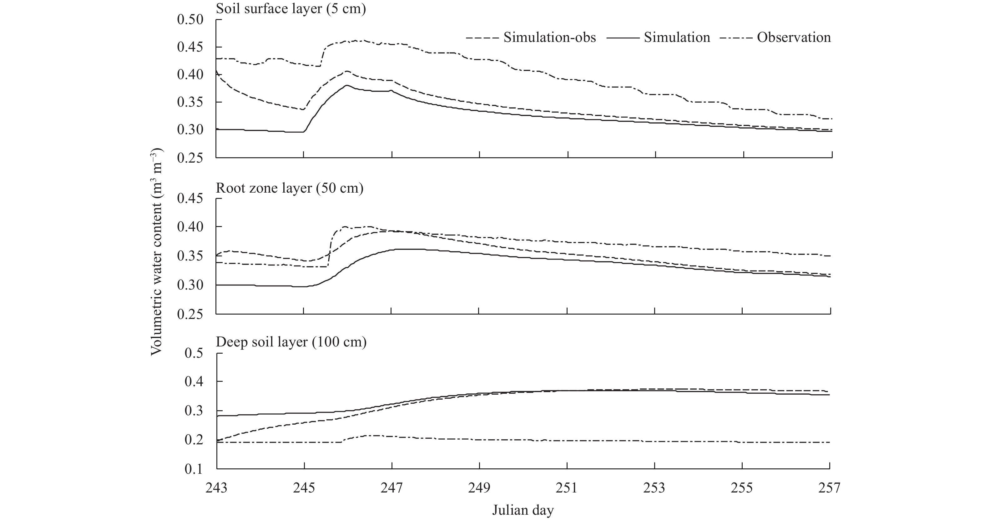
4.1 At Point AAs soil moisture observations were not obtained between days 235 and 237, only the SiB2 model is determined for these three days. First, test whether the amplitude of the model result variation is big at the beginning of the prediction period, then the observed soil moisture at the end of the assimilation period is set to the initial value (Case 0). From the results in Fig. 4, it can be seen that the model is stable after one day in the prediction period, which is to say the model has the memory of one day before stabilization. Then, the influence of assimilated results with different assimilation frequencies and precipitation on soil moisture predictions was investigated.
|
| Figure 4 Soil moisture predictions for Case 0 from 1 to 14 September 2007 (days 244–257) at Point A in Meilin watershed. Simulation-obs refers to the soil moisture simulations based on the observed soil moisture as initial values. |
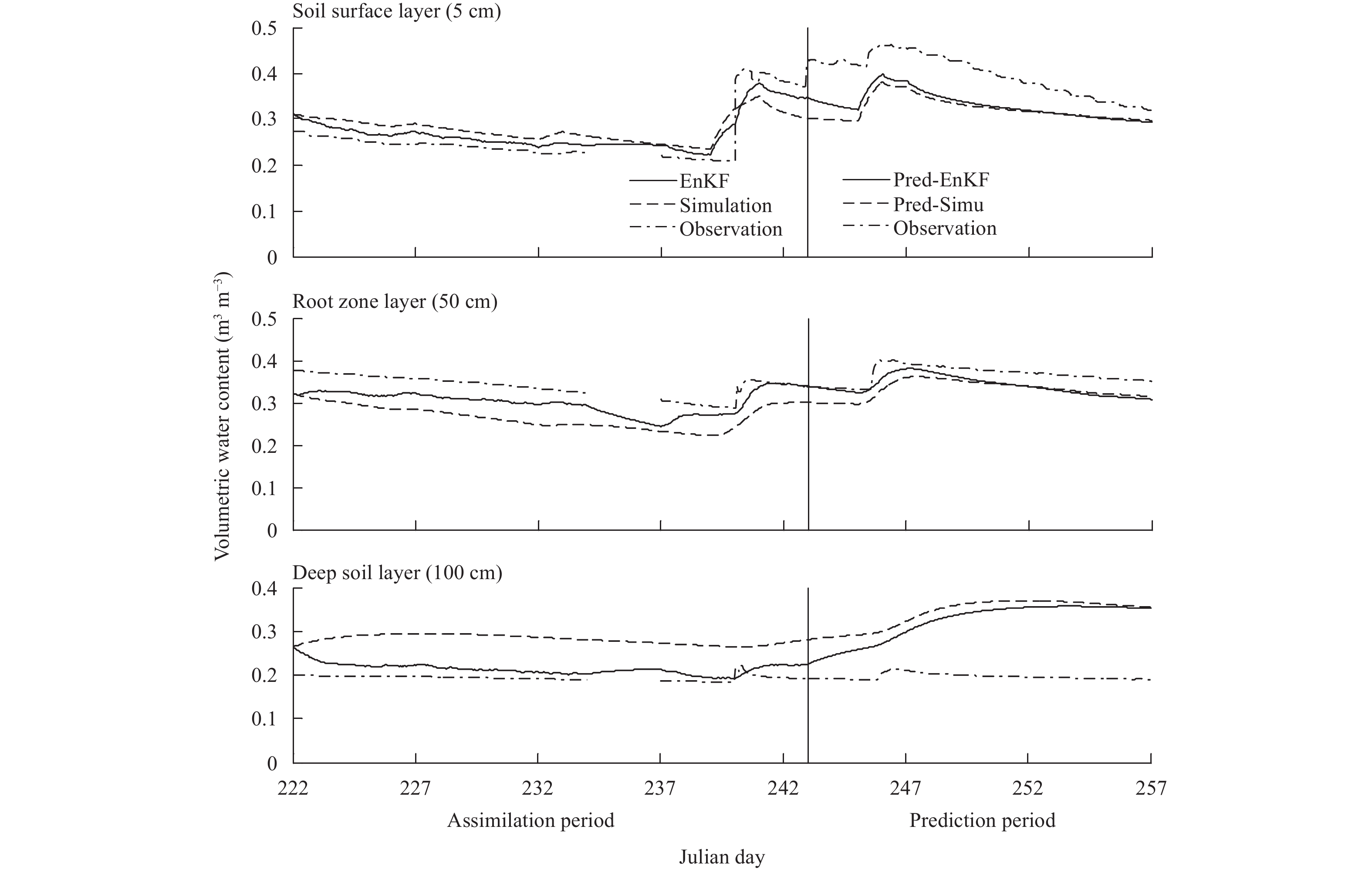
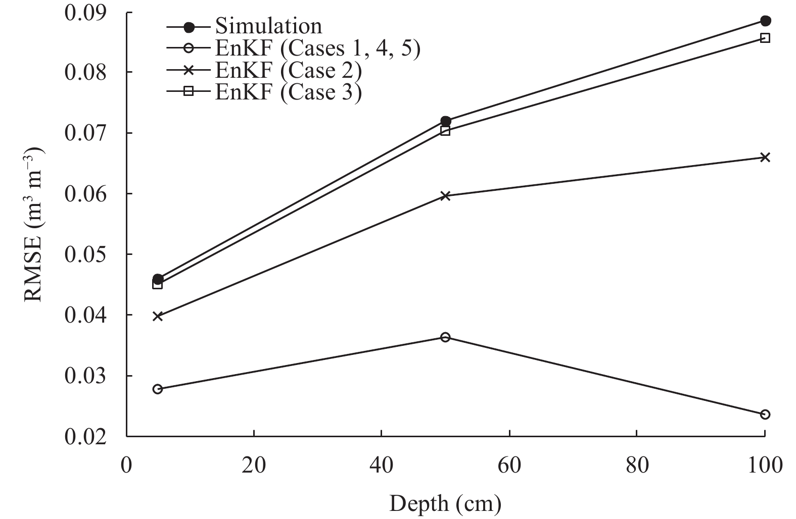
Figure 5 shows the assimilation and prediction results of the soil moisture for Case 1. From Fig. 5, it can be seen that in the assimilation period, EnKF improves the soil moisture simulations at each soil layer. This can also be seen in Fig. 6 that shows the RMSE between the modeled/assimilated and observed soil moistures from 11 to 31 August 2007 (days 223–243) except for the previously mentioned three days without soil moisture observations.
|
| Figure 5 Soil moisture predictions and assimilations for Case 1 from 11 August to 14 September 2007 (days 223–257) at Point A in Meilin watershed. |
|
| Figure 6 RMSE of simulations and assimilations for different cases in the assimilation period (days 223–243) at Point A in Meilin watershed. |
Predictions of the soil moisture from 1 to 14 September 2007 (days 244–257) after the assimilation period were obtained and are shown in Fig. 5. It is noted that the Pred-EnKF results are closer to the observations than the Pred-Simu results in the early portion (e.g., days 244–252 for the surface and root zone layers, 14-day lead-time for the deep soil layer) of the prediction period. However, following that early portion, the Pred-EnKF results become closer to or worse than the Pred-Simu results.
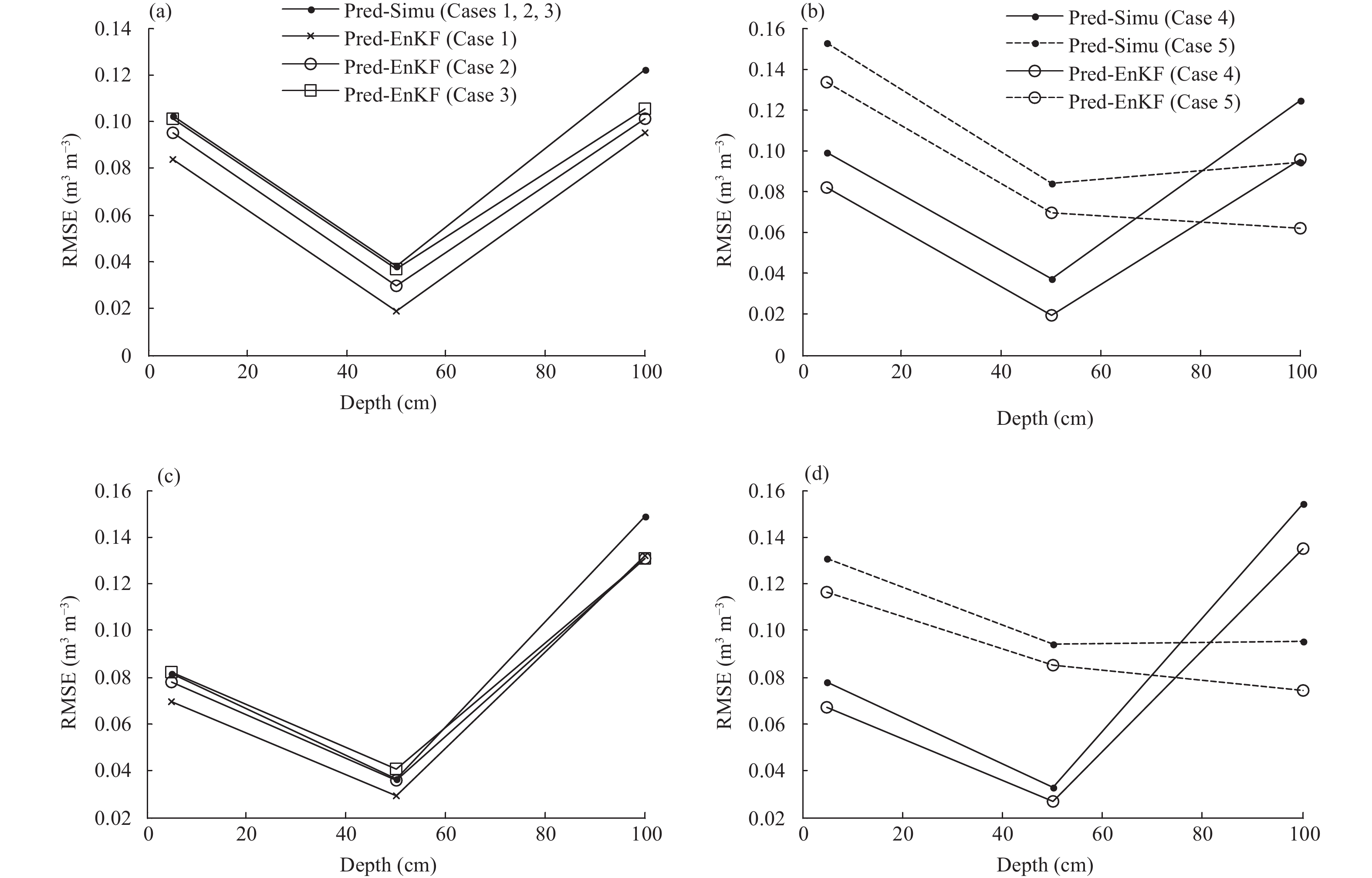
The RMSE of Pred-EnKF results is smaller than that of Pred-Simu results as shown in Fig. 7, indicating that the adequate initial value would be a benefit for improving soil moisture predictions. In addition, for the 7- and 14-day lead-time, the RMSE of Pred-EnKF is significantly smaller than that of Pred-Simu.
|
| Note: Pred-Simu and Pred-EnKF represent predictions followed by the simulated and assimilated values, respectively, at the end time of day 243. Figure 7 RMSE of soil moisture predictions at Point A in Meilin watershed. (a, b) RMSE for 7-day (days 244–250) predictions and (c, d) RMSE for 14-day (days 244–257) predictions at different soil depths. |
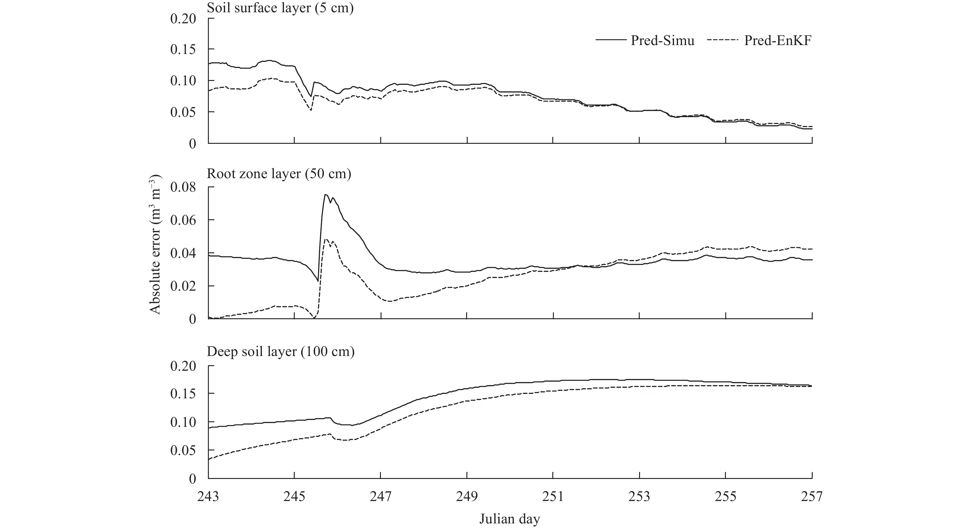
To better highlight the difference in prediction results, the AE values between the Pred-Simu/Pred-EnKF and observations are shown in Fig. 8. The AE values of Pred-EnKF are smaller than those of Pred-Simu for all the three soil layers in the first few days of the prediction period. But at the soil surface and root zone layers, Fig. 8 shows the contrary results for the last several days of prediction period compared to the first few days of this period. The AE values of Pred-Simu and Pred-EnKF generally increase from days 244 to 250 at the root zone and deep soil layers. At the soil surface layer, the AE values of Pred-Simu and Pred-EnKF remain the same for the first two days of the prediction period and decrease from days 246 to 257.
|
| Figure 8 Evolutions of the absolute error (AE) between predicted and observed soil moisture for Case 1 from 1 to 14 September 2007 (days 244–257) at Point A in Meilin watershed. |
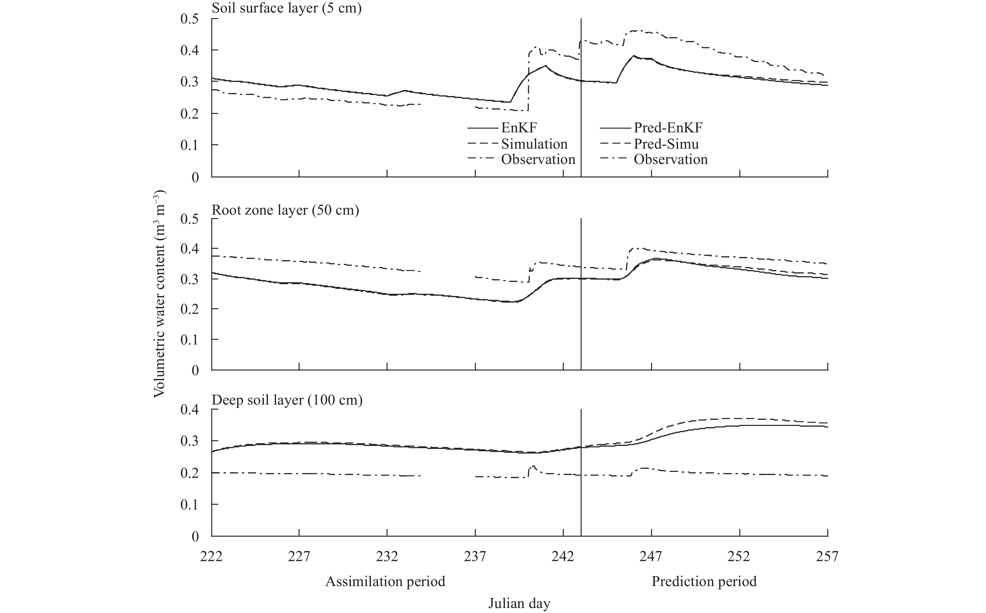
To evaluate the influence of the assimilated results with different assimilation frequencies on soil moisture predictions, the assimilation experiments with other two different frequencies, every three hours (Case 2) and once a day (Case 3), were undertaken. As the results of AE between the Pred-Simu/Pred-EnKF and observations are similar to the results in Fig. 8, the AE results for Cases 2 and 3 are not shown. Figures 9 and 10 show the results of soil moisture assimilations and predictions for Cases 2 and 3, respectively. The results shown in Fig. 9 (Case 2) indicate that EnKF can improve the soil moisture simulations during the assimilation period. Figure 9 also shows that Pred-EnKF is better than Pred-Simu for the first few days of the prediction period and worse in the last few days. The results shown in Fig. 10 (Case 3) indicate that EnKF does not improve the soil moisture simulation significantly at the assimilation period with a daily assimilation frequency. For the prediction period in Case 3, the Pred-EnKF is better than Pred-Simu for approximately the first six days of the prediction period at the first two soil layers. At the deep soil layer, the Pred-EnKF is always better than Pred-Simu for the 14-day lead-time.

|
| Figure 9 As in Fig. 5, but for Case 2 from 11 August to 14 September 2007 (days 223–257) at Point A in Meilin watershed. |
|
| Figure 10 As in Fig. 5, but for Case 3 from 11 August to 14 September 2007 (days 223–257) at Point A in Meilin watershed. |
From Fig. 6, it is noted that the RMSE of assimilations is smaller than that of simulations, which shows that using EnKF improves the soil moisture simulation within the assimilation period for each case. For the prediction period, Fig. 7 shows the RMSE of Pred-EnKF is smaller than that of the Pred-Simu for the 7- or 14-day lead-time for Case 2. However, for Case 3, the RMSE of the Pred-EnKF is smaller than that of the Pred-Simu for the 7-day lead-time for all the three soil layers, but greater than that of the Pred-Simu for the 14-day lead-time at the soil surface and root zone layers.
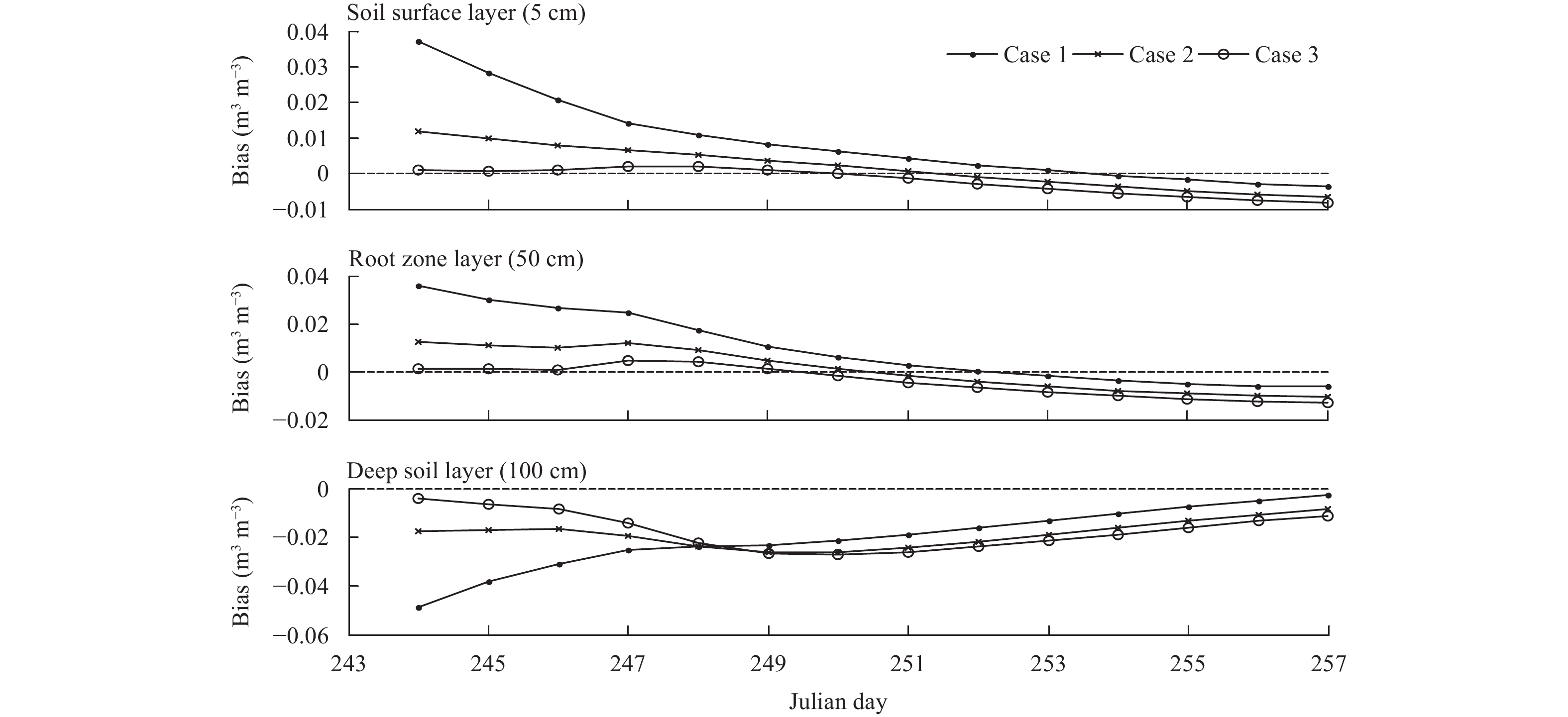
Comparing the results among Cases 1–3, the EnKF performs worse as the assimilation frequency decreases. EnKF can improve the soil moisture simulation significantly for the hourly assimilation, but the improvement is in-significantly for the daily assimilation. This is because, as the assimilation frequency decreases, the optimized soil moisture simulation decreases, which negatively affects the performance of the EnKF. In addition, it can be seen that the assimilated results at the end of the assimilation period deviate further from observations as the assimilation frequency decreases. From the results inFigs. 5, 9, 10, it can be seen that the initial state values (assimilated results at the end of the assimilation period) for the soil moisture prediction are different, which leads to different Pred-EnKF results. It is noted that the Pred-EnKF results become worse from Cases 1 to 3 at the soil surface and root zone layers, but still better than the Pred-Simu results for the first few days of the prediction period. In the deep soil layer, Pred-EnKF results are better than Pred-Simu results for the three cases of the 14-day lead-time. This is likely because the initial values become closer to the simulated soil moisture from Cases 1 to 3, which results in the Pred-EnKF deviating further from observations from Cases 1 to 3 for the first two soil layers. However, for the deep soil layer, the soil moisture is relatively stable, and the initial value is closer to observations than the simulated soil moisture so that the Pred-EnKF is better than Pred-Simu at this layer. Figure 11 shows the daily average bias between the Pred-EnKF and Pred-Simu for Cases 1–3 during the prediction period. From this figure, it can be found that the time when Pred-EnKF is better than Pred-Simu becomes shorter from Cases 1 to 3 for the first two soil layers, i.e., Pred-EnKF is better than Pred-Simu for the 10-, 8-, and 7-day predictions corresponding to Cases 1, 2, and 3, respectively at the soil surface layer, and the 9-, 7-, and 6-day predictions related to Cases 1, 2, and 3, respectively at the root zone layer. A possible reason may be that the different initial values have the same forcing condition in all the three cases. The initial value is closer to the simulated soil moisture in Case 3, which results in the Pred-EnKF farther from observations earlier in the prediction period for Case 3. At the deep soil layer, the daily average bias is relatively stable after Day 247 (precipitation day), which may be ascribed to the stable soil moisture at this layer.
|
| Figure 11 Daily average bias between the Pred-EnKF and Pred-Simu results in the prediction period (days 244–257) for Cases 1–3 at Point A in Meilin watershed. The simulations overestimated the soil moisture at the soil surface and root zone layers, but underestimated at the deep soil layer. Thus, bias > 0 means that Pred-EnKF is better than Pred-Simu at the first two soil layers, and bias < 0 means that Pred-EnKF is better than Pred-Simu at the deep soil layer. |
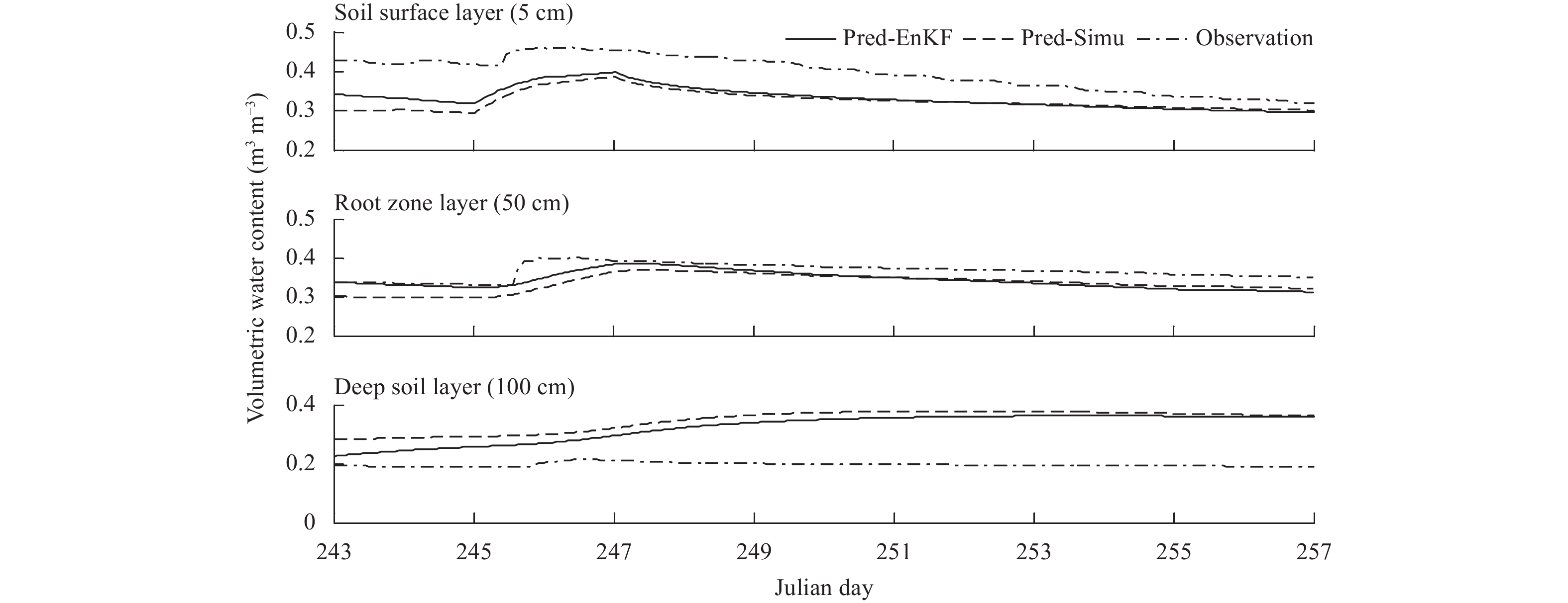
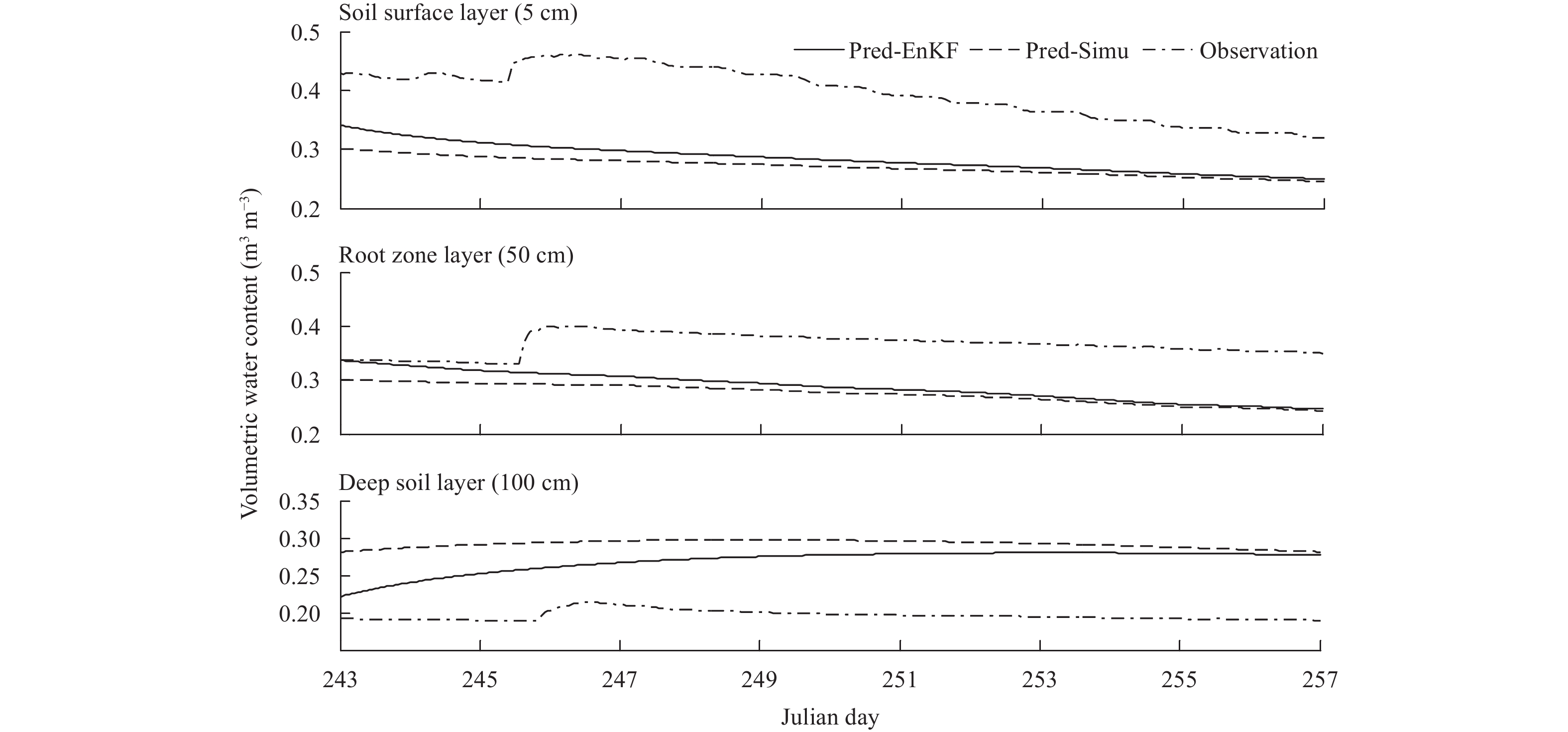
To evaluate the influence of precipitation on soil moisture predictions, the measured precipitation was multiplied by a randomly value generated from a uniform distribution U (0, 2), and zero precipitation were used in the prediction period in Cases 4 and 5. In these two cases, the soil moisture assimilations at the end of the assimilation period with an hourly assimilation frequency are used as the initial values, so the results of soil moisture simulations and assimilations in the assimilation period are not shown, which can be found in Fig. 5. Figures 12 and 13 only show the soil moisture predictions from 1–14 September 2007 (days 244–257) for Cases 4 and 5. The Pred-EnKF is closer to observations compared to Pred-Simu for the first few days of the prediction period (Fig. 12), but contrary for the last few days at the first two soil layers. At the deep soil layer, the Pred-EnKF is closer to observations than Pred-Simu. For Case 5, the Pred-EnKF is also closer to observations than Pred-Simu at all the three soil layers (Fig. 13). Figure 7 shows that the RMSE of Pred-EnKF is smaller than that of Pred-Simu for the 7- and 14-day lead times.
|
| Figure 12 Soil moisture predictions for Case 4 from 1 to 14 September 2007 (days 244–257) at Point A in Meilin watershed. |
|
| Figure 13 As in Fig. 12, but for Case 5 from 1 to 14 September 2007 (days 244–257) at Point A in Meilin watershed. |
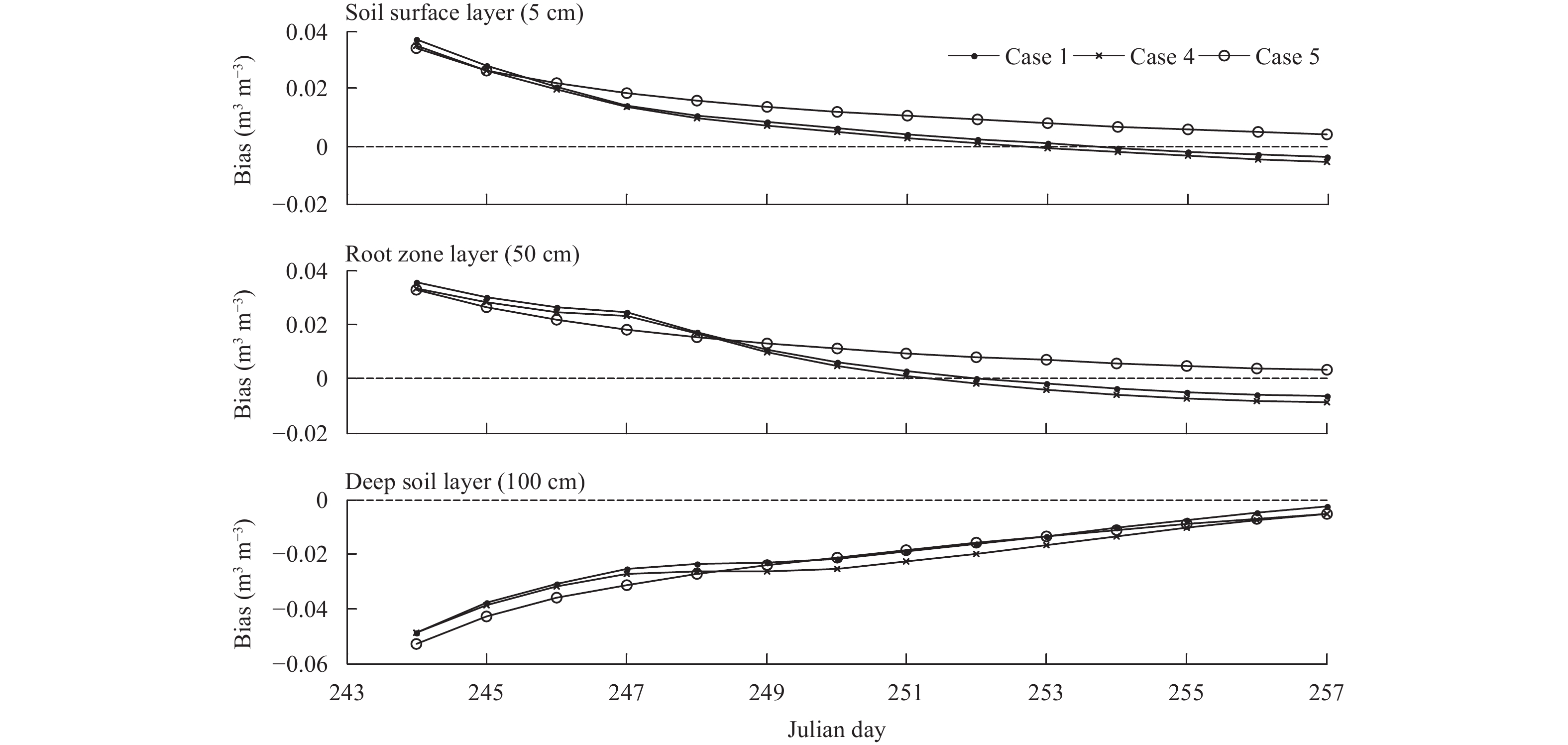
By comparing the results for Cases 1, 4, and 5, the Pred-EnKF is closer to observations than Pred-Simu for the first few days of the prediction period at the first two soil layers when there is precipitation. However, for the period without precipitation, the Pred-EnKF is better than Pred-Simu for the 14-day lead-time. This can be seen in Fig. 14 that shows the daily average bias between the Pred-EnKF and Pred-Simu for Cases 1, 4, and 5 for the prediction period. A possible reason may be that the Pred-EnKF and Pred-Simu increase with the occurrence of precipitation, and following a day of precipitation, the Pred-EnKF and Pred-Simu decrease quickly with large evapotranspiration. This results in the Pred-EnKF and Pred-Simu becoming closer to each other, and even the Pred-EnKF is worse than Pred-Simu for the last few days of the prediction period for Cases 1 and 4 at the soil surface and root zone layers. For Case 5, as there is no precipitation, the Pred-EnKF and Pred-Simu decrease gradually, and Pred-EnKF becomes closer to Pred-Simu during the prediction period.
|
| Figure 14 As in Fig. 11, but for Cases 1, 4, and 5. |
Point B in the Meilin watershed provided observation data that were collected above the bottom of the watershed from 1 December 2008 to 14 February 2009. This is used to examine if results vary with the location or time period by comparison to Point A. At this point, only four cases, i.e., Cases 6–9, are considered.
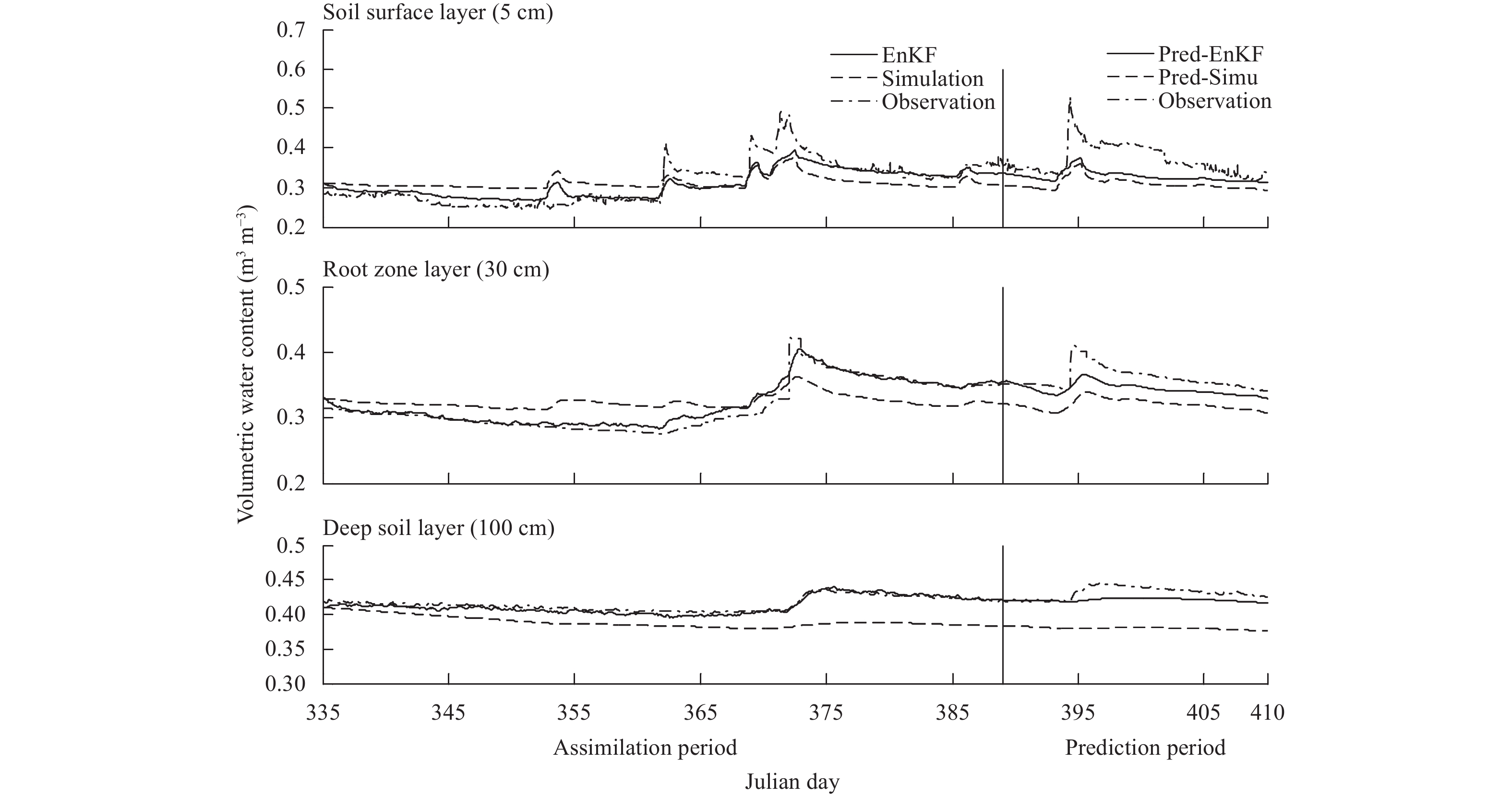
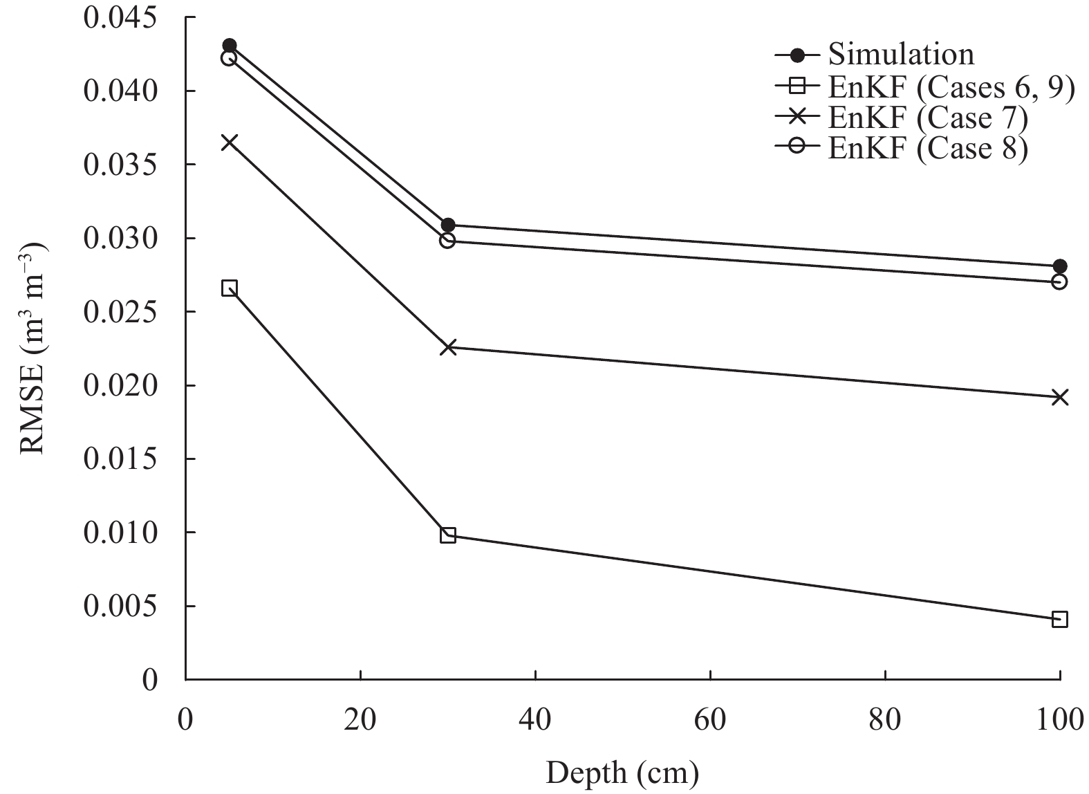
For Case 6, the soil moisture assimilation and prediction results are shown in Fig. 15, in which shows the soil moisture assimilation results (from 1 December 2008 to 24 January 2009) are closer to observations than simulations in the assimilation period for all the soil layers as demonstrated by the RMSE results between the modeled/assimilated and observed soil moistures of the assimilation period in Fig. 16.
|
| Figure 15 As in Fig. 5, but for Case 6 from 1 December 2008 to 14 February 2009 (days 335–410) at Point B in Meilin watershed. |
|
| Figure 16 RMSE of simulations and assimilations for different cases in the assimilation period (days 335–389) at Point B in Meilin watershed. |
Figure 15 also shows the soil moisture predictions from 25 January to 14 February 2009 (days 390–410), and displays that the Pred-EnKF results are significantly closer to observations than Pred-Simu results in the 21-day prediction period for Point B. Thus, the RMSE and AE of the soil moisture results for Point B in the prediction period are not shown.
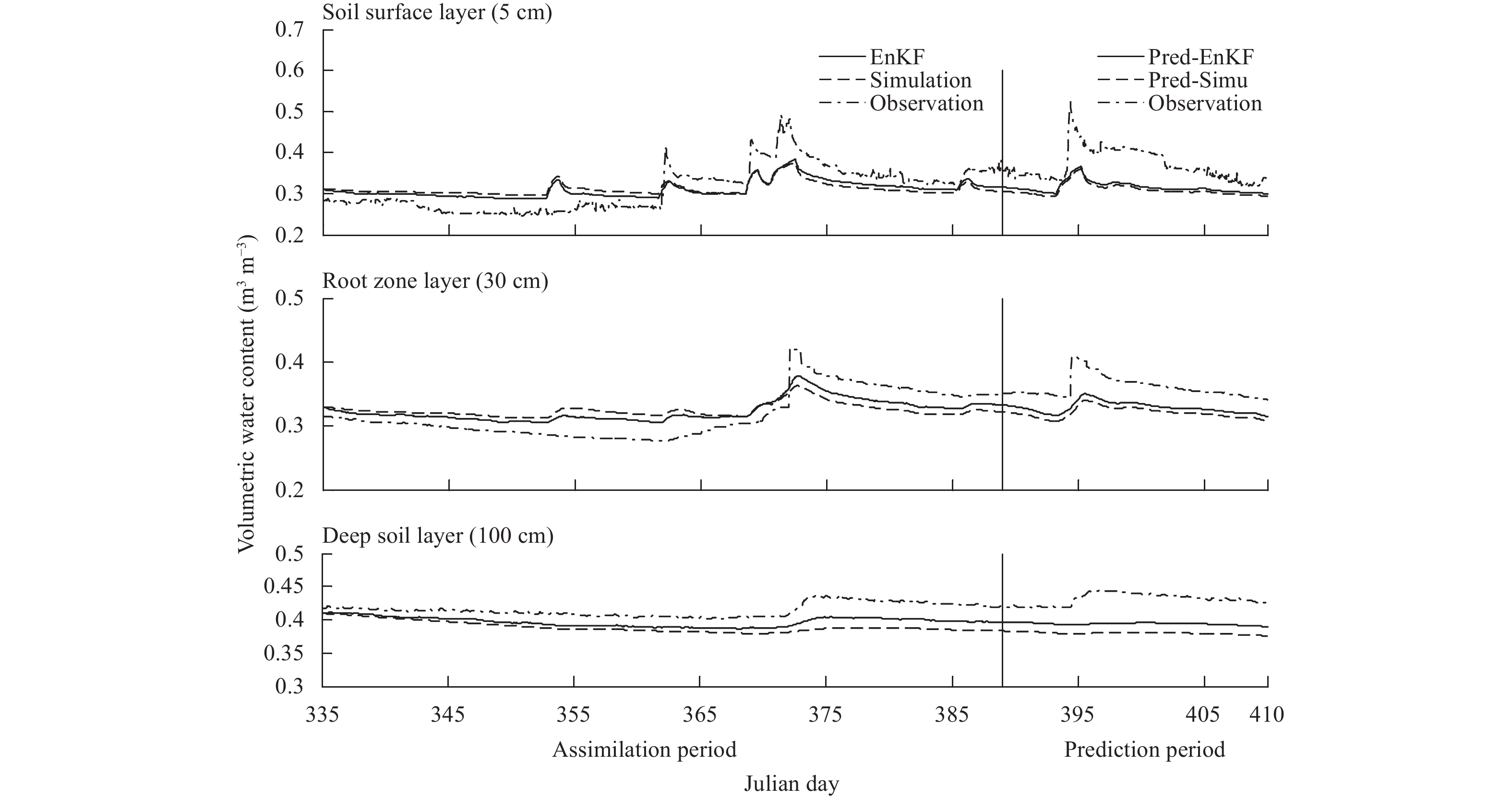
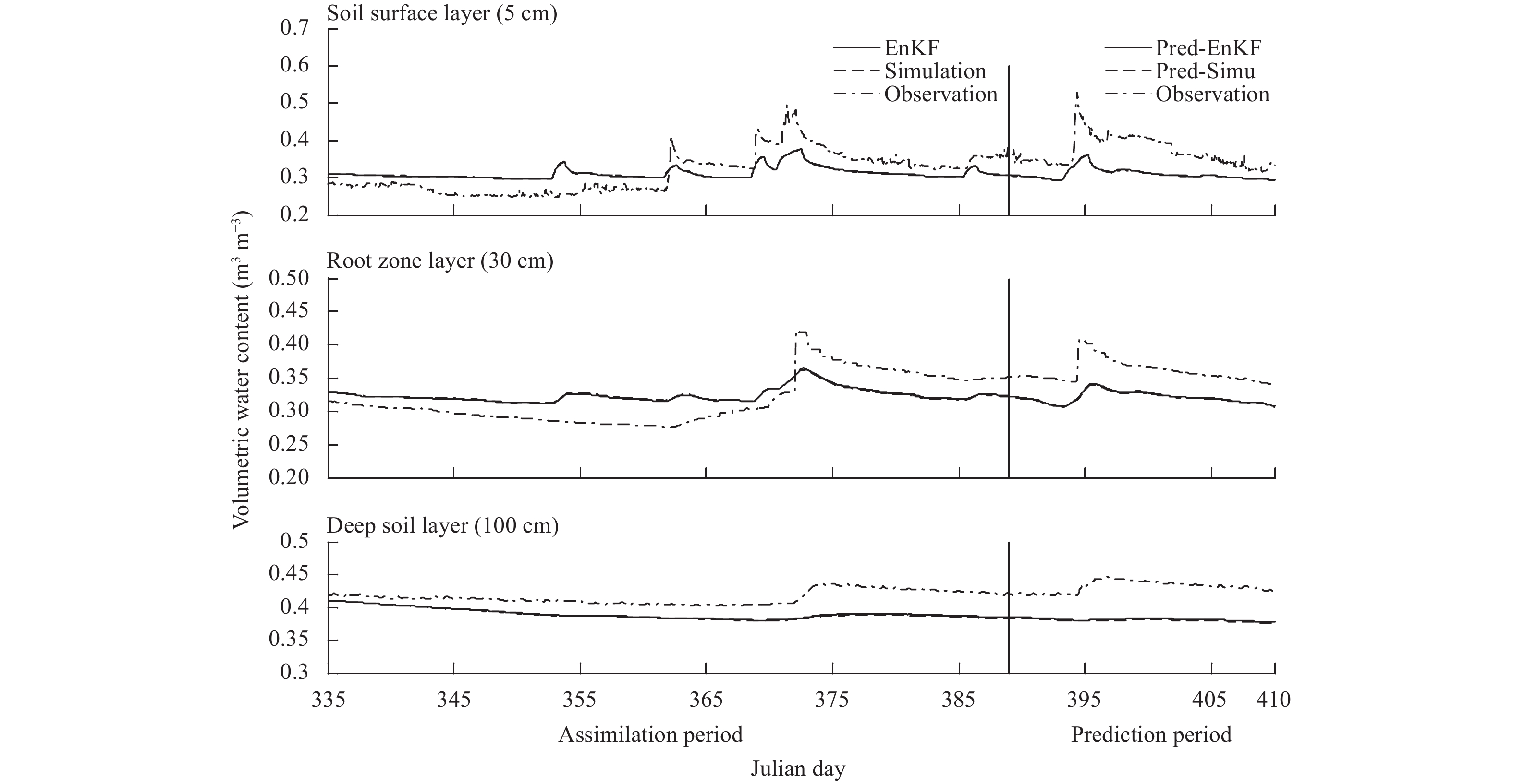
Similar to the experiment designs at Point A, the assimilation experiments with frequencies every three hours (Case 7) and once a day (Case 8) at Point B were performed. The soil moisture assimilations and predictions for Cases 7 and 8 are shown in Figs. 17, 18, respectively, which show that the soil moisture simulations are improved by the EnKF in the assimilation per-iod, which can also be seen from Fig. 16. Also, the Pred-EnKF results are closer to observations than simulations for all the soil layers during the entire prediction period. However, the daily assimilation experiment (Fig. 18) leads to the Pred-EnKF being better than Pred-Simu, but not obvious.
|
| Figure 17 As in Fig. 5, but for Case 7 from 1 December 2008 to 14 February 2009 (days 335–410) at Point B in Meilin watershed. |
|
| Figure 18 As in Fig. 5, but for Case 8 from 1 December 2008 to 14 February 2009 (days 335–410) at Point B in Meilin watershed. |
By comparing the results for Cases 6 to 8, it is found that the results are similar for the assimilation period as discussed in Section 4.1. However, different to the results in Section 4.1, the Pred-EnKF results are all better than Pred-Simu results for the three soil layers during the 21-day prediction period for Cases 6 to 8. This may be because Point B is located at the bottom (elevation: about 6 m) of Meilin watershed, which is a humid area, and the prediction period is in winter, so the daily evapotranspiration is small, and the water table depth is fairly shallow, which may result in small infiltration.
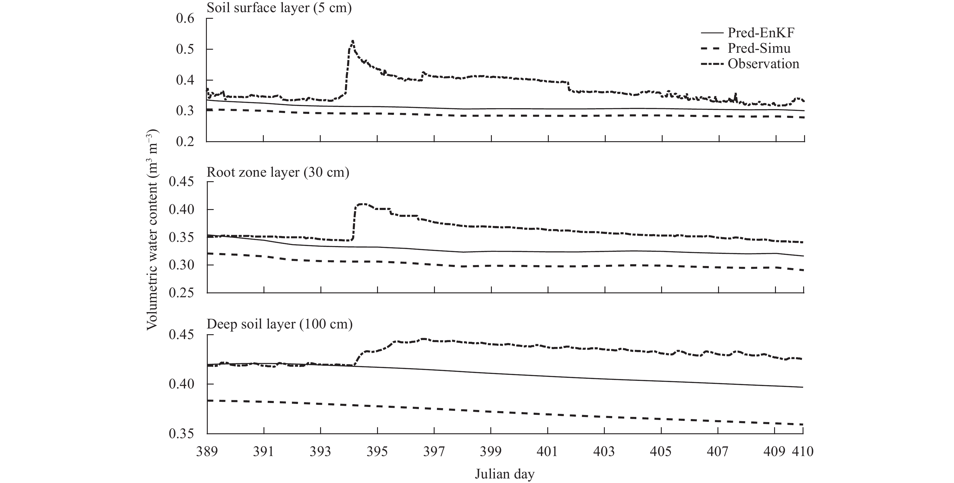
Comparison between Cases 1 and 4 in Section 4.1 shows that the measured precipitation times a random value has little influence on the change of the soil moisture prediction. Thus, only the zero precipitation case is used during the prediction period for Point B in Case 9 to analyze the influence of precipitation on soil moisture predictions. Figure 19 shows the soil moisture predictions from 25 January to 14 February 2009 (days 390–410), based on initial state values following the hourly frequency assimilation experiment. It is noted that Pred-EnKF results are better than those of Pred-Simu at all the soil layers for the 21-day prediction period. Since the precipitation is zero for the prediction period, the Pred-EnKF and Pred-Simu are all stable for all the three soil layers.
|
| Figure 19 As in Fig. 12, but for Case 9 from 25 January to 14 February 2009 (days 390–410) at Point B in Meilin watershed. |
By comparing the results in Cases 6 and 9, it can be found that the Pred-EnKF is significantly closer to observations than Pred-Simu in the prediction period for the three soil layers. The soil moisture predictions are stable for Case 9 at all the soil layers due to the lack of precipitation and low evapotranspiration in winter.
By comparing the results in Sections 4.1 and 4.2, it is noted that the Pred-EnKF is better than Pred-Simu for the early portion of the summer prediction period at Point A. However, for Point B, the Pred-EnKF is closer to observations than Pred-Simu for the 21-day winter prediction period. A possible reason may be that the high daily evapotranspiration and larger infiltrated water content exist during the summer prediction period at Point A (top of the watershed), so the soil moisture content changes significantly. On the other hand, the soil moisture content is stable at Point B (bottom of the watershed) in the winter prediction period due to the low evapotranspiration and lower infiltrated water content.
5 ConclusionsThis study investigated the influence of the assimilated soil moisture with different assimilation frequencies before the current time and precipitation on the soil moisture predictions based on the SiB2 model and EnKF. Ten cases are considered and evaluated by using data from the Meilin watershed, eastern China.
For the summer prediction period with a deeper water table depth (Point A), the assimilation results with different assimilation frequencies before the current time can influence the soil moisture predictions in the future. Based on the initial value (assimilated results at the end of assimilation period), a higher assimilation frequency gives better soil moisture predictions with a long lead-time. For a low assimilation frequency (e.g., once a day), the EnKF does not improve soil moisture simulations significantly in the assimilation period.
Soil moisture predictions are affected by precipitation. And the predictions are better for a short lead-time when there is precipitation, and better for a long lead-time when there is no precipitation, based on the same initial value.
For the winter prediction period with a lower water table depth (Point B), soil moisture predictions are better through the whole prediction period based on the initial value. A high assimilation frequency gives better soil moisture predictions. Also, the precipitation does not strongly influence soil moisture predictions for Point B as observed for Point A.
| Balsamo, G., J. F. Mahfouf, S. Bélair, et al., 2007: A land data assimilation system for soil moisture and temperature: An information content study. J. Hydrometeorol., 8, 1225–1242. DOI:10.1175/2007JHM819.1 |
| Dai, Y. J., X. B. Zeng, R. E. Dickinson, et al., 2003: The common land model. Bull. Amer. Meteor. Soc., 84, 1013–1024. DOI:10.1175/BAMS-84-8-1013 |
| Decker, M., and X. B. Zeng, 2009: Impact of modified Richards equation on global soil moisture simulation in the Community Land Model (CLM3.5). J. Adv. Model. Earth Syst., 1, 5. DOI:10.3894/JAMES.2009.1.5 |
| Dumedah, G., and P. Coulibaly, 2013: Evaluating forecasting performance for data assimilation methods: The ensemble Kalman filter, the particle filter, and the evolutionary-based assimilation. Adv. Water Resour., 60, 47–63. DOI:10.1016/j.advwatres.2013.07.007 |
| Dumedah, G., and J. P. Walker, 2014: Assessment of land surface model uncertainty: A crucial step towards the identification of model weaknesses. J. Hydrol., 519, 1474–1484. DOI:10.1016/j.jhydrol.2014.09.015 |
| Dumedah, G., and J. P. Walker, 2017: Assessment of model behavior and acceptable forcing data uncertainty in the context of land surface soil moisture estimation. Adv. Water Resour., 101, 23–36. DOI:10.1016/j.advwatres.2017.01.001 |
| Evensen, G., 1994: Sequential data assimilation with a nonlinear quasi-geostrophic model using Monte Carlo methods to forecast error statistics. J. Geophys. Res. Oceans, 99, 10143–10162. DOI:10.1029/94JC00572 |
| Famiglietti, J. S., and E. F. Wood, 1994: Multiscale modeling of spatially variable water and energy balance process. Water Resour. Res., 30, 3061–3078. DOI:10.1029/94WR01498 |
| Fu, X. L., Z. B. Yu, L. F. Luo, et al., 2014: Investigating soil moisture sensitivity to precipitation and evapotranspiration errors using SiB2 model and ensemble Kalman filter. Stoch. Environ. Res. Risk Assess., 28, 681–693. DOI:10.1007/s00477-013-0781-3 |
| Fu, X. L., L. F. Luo, M. Pan, et al., 2018a: Evaluation of TOPMODEL-based land surface–atmosphere transfer scheme (TOPLATS) through a soil moisture simulation. Earth Interact., 22, 1–19. DOI:10.1175/EI-D-17-0037.1 |
| Fu, X. L., Z. B. Yu, Y. J. Ding, et al., 2018b: Analysis of influence of observation operator on sequential data assimilation through soil temperature simulation with common land mo-del. Water Sci. Eng., 11, 196–204. DOI:10.1016/j.wse.2018.09.003 |
| Han, X. J., and X. Li, 2008: An evaluation of the nonlinear/non-Gaussian filters for the sequential data assimilation. Remote Sens. Environ., 112, 1434–1449. DOI:10.1016/j.rse.2007.07.008 |
| Han, X. J., H. J. H. Franssen, C. Montzka, et al., 2014: Soil moisture and soil properties estimation in the Community Land Model with synthetic brightness temperature observations. Water Resour. Res., 50, 6081–6105. DOI:10.1002/2013WR014586 |
| Heathman, G. C., P. J. Starks, L. R. Ahuja, et al., 2003: Assimilation of surface soil moisture to estimate profile soil water content. J. Hydrol., 279, 1–17. DOI:10.1016/S0022-1694(03)00088-X |
| Heemink, A. W., M. Verlaan, and J. Segers, 2001: Variance reduced ensemble Kalman filtering. Mon. Wea. Rev., 129, 1718–1728. DOI:10.1175/1520-0493(2001)129<1718:VREKF>2.0.CO;2 |
| Houtekamer, P. L., and H. L. Mitchell, 2001: A sequential ensemble Kalman filter for atmospheric data assimilation. Mon. Wea. Rev., 129, 123–137. DOI:10.1175/1520-0493(2001)129<0123:ASEKFF>2.0.CO;2 |
| Huang, C. L., and X. Li, 2004: A review of land data assimilation system. Remote Sens. Technol. Appl., 19, 424–430. DOI:10.3969/j.issn.1004-0323.2004.05.026 |
| Huang, C. L., X. Li, L. Lu, et al., 2008: Experiments of one-dimensional soil moisture assimilation system based on ensemble Kalman filter. Remote Sens. Environ., 112, 888–900. DOI:10.1016/j.rse.2007.06.026 |
| Jackson, T. J., D. M. Le Vine, A. Y. Hsu, et al., 1999: Soil moisture mapping at regional scales using microwave radiometry: The southern great plains hydrology experiment. IEEE Trans. Geosci. Remote Sens., 37, 2136–2151. DOI:10.1109/36.789610 |
| Kalman, R. E., 1960: A new approach to linear filtering and prediction problems. J. Basic Eng., 82, 35–45. DOI:10.1115/1.3662552 |
| Koster, R. D., P. A. Dirmeyer, Z. C. Guo, et al., 2004: Regions of strong coupling between soil moisture and precipitation. Science, 305, 1138–1140. DOI:10.1126/science.1100217 |
| Lai, X., J. Wen, S. X. Cen, et al., 2014: Numerical simulation and evaluation study of soil moisture over China by using CLM4.0 model. Chinese J. Atmos. Sci., 38, 499–512. DOI:10.3878/j.issn.1006-9895.1401.13194 |
| Li, F. Q., W. T. Crow, and W. P. Kustas, 2010: Towards the estimation root-zone soil moisture via the simultaneous assimilation of thermal and microwave soil moisture retrievals. Adv. Water Resour., 33, 201–214. DOI:10.1016/j.advwatres.2009.11.007 |
| Liang, X., D. P. Lettennmaier, E. F. Wood, et al., 1994: A simple hydrologically based model of land surface water and energy fluxes for general circulation models. J. Geophys. Res. Atmos., 99, 14415–14428. DOI:10.1029/94JD00483 |
| Lievens, H., G. J. M. De Lannoy, A. Al Bitar, et al., 2016: Assimilation of SMOS soil moisture and brightness temperature products into a land surface model. Remote Sens. Environ., 180, 292–304. DOI:10.1016/j.rse.2015.10.033 |
| Liu, D., A. K. Mishra, and Z. B. Yu, 2016: Evaluating uncertainties in multi-layer soil moisture estimation with support vector machines and ensemble Kalman filtering. J. Hydrol., 538, 243–255. DOI:10.1016/j.jhydrol.2016.04.021 |
| Liu, H. R., F. Y. Lu, Z. Y. Liu, et al., 2016: Assimilating atmosphere reanalysis in coupled data assimilation. J. Meteor. Res., 30, 572–583. DOI:10.1007/s13351-016-6014-1 |
| Luo, L. F., A. Robock, K. E. Mitchell, et al., 2003: Validation of the North American land data assimilation system (NLDAS) retrospective forcing over the southern Great Plains. J. Geophys. Res. Atmos., 108, 8843. DOI:10.1029/2002JD003246 |
| Luo, S. Q., X. W. Fang, S. H. Lyu, et al., 2017: Improving CLM4.5 simulations of land–atmosphere exchange during freeze–thaw processes on the Tibetan Plateau. J. Meteor. Res., 31, 916–930. DOI:10.1007/s13351-017-6063-0 |
| Lyu, H. S., Z. B. Yu, R. Horton, et al., 2011a: Multi-scale assimilation of root zone soil water predictions. Hydrol. Processes, 25, 3158–3172. DOI:10.1002/hyp.8034 |
| Lyu, H. S., Z. B. Yu, Y. H. Zhu, et al., 2011b: Dual state-parame-ter estimation of root zone soil moisture by optimal parame-ter estimation and extended Kalman filter data assimilation. Adv. Water Resour., 34, 395–406. DOI:10.1016/j.advwatres.2010.12.005 |
| Milly, P. C. D., J. Betancourt, M. Falkenmark, et al., 2008: Stationarity is dead: Whither water management?. Science, 319, 573–574. DOI:10.1126/science.1151915 |
| Monteith, J. L., 1973: Principles of Environmental Physics. Edward Arnold, London, 242 pp. |
| Moradkhani, H., S. Sorooshian, H. V. Gupta, et al., 2005: Dual state-parameter estimation of hydrological models using ensemble Kalman filter. Adv. Water Resour., 28, 135–147. DOI:10.1016/j.advwatres.2004.09.002 |
| Oleson, K. W., Y. J. Dai, G. B. Bonan, et al., 2004: Technical Description of the Community Land Model (CLM). NCAR Technical Note NCAR/TN-461+STR, National Center for Atmospheric Research, Boulder, CO, doi: 10.5065/D6N877R0. |
| Rodell, M., P. R. Houser, U. Jambor, et al., 2004: The global land data assimilation system. Bull. Amer. Meteor. Soc., 85, 381–394. DOI:10.1175/BAMS-85-3-381 |
| Schaake, J. C., Q. Y. Duan, V. Koren, et al., 2004: An intercomparison of soil moisture fields in the North American Land Data Assimilation System (NLDAS). J. Geophys. Res. Atmos., 109, D01S90. DOI:10.1029/2002JD003309 |
| Sellers, P. J., D. A. Randall, G. J. Collatz, et al., 1996: A revised land surface parameterization (SiB2) for atmospheric GCMs. Part I: Model formulation. J. Climate, 9, 676–705. DOI:10.1175/1520-0442(1996)009<0676:ARLSPF>2.0.CO;2 |
| Shi, J. C., L. M. Jiang, L. X. Zhang, et al., 2006: Physically based estimation of bare-surface soil moisture with the passive radiometers. IEEE Trans. Geosci. Remote Sens., 44, 3145–3153. DOI:10.1109/TGRS.2006.876706 |
| Vrugt, J. A., H. V. Gupta, B. O. Nualláin, et al., 2006: Real-time data assimilation for operational ensemble streamflow forecasting. J. Hydrometeorol., 7, 548–565. DOI:10.1175/JHM504.1 |
| Wang, G. J., D. Chyi, L. Wang, et al., 2016: Soil moisture retrie-val over Northeast China based on microwave brightness temperature of FY3B satellite and its comparison with other datasets. Chinese J. Atmos. Sci., 40, 792–804. DOI:10.3878/j.issn.1006-9895.1509.15207 |
| Weerts, A. H., and G. Y. H. El Serafy, 2006: Particle filtering and ensemble Kalman filtering for state updating with hydrologi-cal conceptual rainfall-runoff models. Water Resour. Res., 42, W09403. DOI:10.1029/2005WR004093 |
| Western, A. W., and G. Blöschl, 1999: On the spatial scaling of soil moisture. J. Hydrol., 217, 203–224. DOI:10.1016/S0022-1694(98)00232-7 |
| Whitaker, J. S., and T. M. Hamill, 2002: Ensemble data assimilation without perturbed observations. Mon. Wea. Rev., 130, 1913–1924. DOI:10.1175/1520-0493(2002)130<1913:EDAWPO>2.0.CO;2 |
| Xiang, L., W. W. Ling, Y. S. Zhu, et al., 2016: Self-adaptive Green-Ampt infiltration parameters obtained from measured moisture processes. Water Sci. Eng., 9, 256–264. DOI:10.1016/j.wse.2016.05.001 |
| Xie, X. H., and D. X. Zhang, 2010: Data assimilation for distributed hydrological catchment modeling via ensemble Kalman filter. Adv. Water Resour., 33, 678–690. DOI:10.1016/j.advwatres.2010.03.012 |
| Yeh, T. C., R. T. Wetherald, and S. Manabe, 1984: The effect of soil moisture on the short-term climate and hydrology change—A numerical experiment. Mon. Wea. Rev., 112, 474–490. DOI:10.1175/1520-0493(1984)112<0474:TEOSMO>2.0.CO;2 |
| Yu, Z. B., T. N. Carlson, E. J. Barron, et al., 2001: On evaluating the spatial–temporal variation of soil moisture in the Susquehanna River Basin. Water Resour. Res., 37, 1313–1326. DOI:10.1029/2000WR900369 |
| Yu, Z. B, X. L. Fu, L. F. Luo, et al., 2014a: One-dimensional soil temperature simulation with Common Land Model by assimilating in situ observations and MODISLST with the ensemble particle filter. Water Resour. Res., 50, 6950–6965. DOI:10.1002/2012WR013473 |
| Yu, Z. B., X. L. Fu, H. S. Lyu, et al., 2014b: Evaluating ensemble Kalman, particle, and ensemble particle filters through soil temperature prediction. J. Hydrol. Eng., 19, 0414027. DOI:10.1061/(ASCE)HE.1943-5584.0000976 |
 2019, Vol. 33


