1 Introduction

Due to limited grid resolution in large-scale weather and climate numerical models, surface turbulent (momentum, sensible, and latent heat) fluxes in the surface layer are usually parameterized in the models. Since the surface fluxes are essential components of land–atmosphere interactions and associated with exchange and transport of mass and momentum, the validity and precision of the surface layer parameterization schemes are key factors for the performance of the weather and climate numerical models. Therefore, it is necessary to investigate the performance of the surface layer parameterization against observations.

Usually the evaluation of the surface layer parameterization against observational data is conducted by either online or offline approach. There have been numbers of studies for online evaluation (e.g., Betts et al., 1997; Chen et al., 1997; Lee et al., 2010; Anurose and Subrahamanyam, 2014), i.e., numerical models employing surface layer parameterization schemes are run and then the simulation results of the numerical models are evaluated against observations to investigate the impact of the surface layer parameterization on the simulation. Since the meteorological quantities that drive the surface layer parameterization schemes to output surface turbulent fluxes are predicted by the numerical models themselves, errors in the meteorological quantities will definitely contribute to errors in the parameterized turbulent fluxes. Thus, in the case, online evaluation is not helpful in evaluating the surface layer parameterization exclusively.

In offline evaluation, the surface layer parameterization schemes calculating the turbulent fluxes are driven by the mean meteorological quantities measured in-situ, and then the parameterized turbulent fluxes are evaluated against the surface turbulent fluxes measured at the same site. Using this approach, the surface layer parameterization can be directly evaluated against observations without errors that may be introduced by other physical processes like boundary layer mixing, clouds, radiation, and model dynamics.

Due to lack of long-term continuous observations of surface turbulent fluxes, direct offline evaluation of surface layer parameterization against observations has been limited until recent years. For example, Cassano et al. (2001) evaluated seven surface layer parameterization schemes against observations in Antarctica; Sodemann and Foken (2003) evaluated a parameterization for turbulent fluxes of momentum and heat in stably stratified surface layers against predictions by another parameterization as well as against observations in Antarctica; Poulos and Burns (2003) evaluated bulk Ri-based surface layer flux formulas for stable and very stable conditions using CASES-99 data observed over the relatively flat terrain of southeast Kansas in the United States; Freedman and Ek (2004) also used CASES-99 observational data to test NCEP operational surface layer parameterizations for stable conditions; Castelli et al. (2011) investigated surface-layer parameterizations against urban surface layer observations in Turin city, Italy; Liu et al. (2013, 2017) evaluated the performance of six surface layer parameterization schemes employed in large-scale weather and climate numerical models using long-term ARM (Atmospheric Radiation Measurement) observational data measured in the southern Great Plains in the United States; Wang et al. (2013) evaluated four turbulent surface flux parameterization schemes over tall grass in a Beijing suburb, northern China; Tassone and Ek (2015) used Ameriflux data for verification of surface layer parameterizations; Katz and Zhu (2017) evaluated a surface layer parameterization scheme using observational data collected at a station off the coast of Gulf of Mexico.

Most of the offline evaluations were conducted against field data observed in the United States due to the availability of long-term continuous flux observational data there. Since different regions may have different climate and land surface conditions, with which the performance of the surface layer parameterization may be implicated, for the consideration of diversity of research sites and regions, evaluation of two surface layer parameterization schemes for the momentum and sensible heat flux is conducted in this study against long-term continuous surface turbulent flux data observed at two sites in the suburb of Nanjing, eastern China to investigate their performance there.

Since all surface layer parameterization schemes have the same framework of theory (i.e., Monin and Obukhov, 1954), the main differences between the different surface layer schemes lie in the expressions of the stability functions ${\varPsi _{\rm m}}$ and ${\varPsi _{\rm h}}$ , which were developed by different authors for their respective surface layer schemes. Among the surface layer schemes, the Pleim–Xiu (PX) scheme (Pleim and Xiu, 1995, 2003; Xiu and Pleim, 2001; Pleim, 2006) employed in the WRF (Weather Research and Forecasting) model (Skamarock et al., 2008) and the scheme employed in the NCAR Community Atmosphere Model (hereafter named CAM scheme; Collins et al., 2004) are two of those that do not employ iteration algorithm and thus are computationally efficient and time-saving. In this study, we select the PX and CAM schemes to evaluate the performance of the momentum and sensible heat flux parameterization in the surface layer and investigate the difference between the parameterization and observation.

In Section 2, the PX and CAM surface layer parameterization schemes are described. In Section 3, the observational sites and data that the evaluation is against are discussed. The evaluation results are analyzed in Section 4. The study is concluded in Section 5.

2 Formulae

Based on the Monin and Obukhov (1954), the momentum flux represented by the friction velocity ( ${u_*}$ ) and the sensible heat flux (SHF) are parameterized as those suggested by Stull (1988).

${u_*} = \dfrac{{kU}}{{\ln \left({\dfrac{z}{{{z_0}}}} \right) - {\varPsi _{\rm m}}\left({\dfrac{z}{L}} \right) + {\varPsi _{\rm m}}\left({\dfrac{{{z_0}}}{L}} \right)}}, $

(1)

${\rm{SHF}} = \rho {c_p}\overline {w'\theta '} = \rho {c_p}\dfrac{{{k^2}U\left({{\theta _0} \!-\! \theta } \right)}}{{\left[ {\ln \left({\dfrac{z}{{{z_0}}}} \right) \!-\! {\varPsi _{\rm m}}\left({\dfrac{z}{L}} \right) \!+\! {\varPsi _{\rm m}}\left({\dfrac{{{z_0}}}{L}} \right)} \right]{\kern 1pt} \! \left[ {\ln \left({\dfrac{z}{{{z_0}}}} \right) \!-\! {\varPsi _{\rm h}}\left({\dfrac{z}{L}} \right) \!+\! {\varPsi _{\rm h}}\left({\dfrac{{{z_0}}}{L}} \right)} \right]}}, $

(2)

where $k$ is the von Kármán constant generally assumed to be 0.4, $\rho $ is the density of air, ${c_p}$ is the specific heat of air at constant pressure, $z$ is the height above ground, ${z_0}$ is the aerodynamical roughness length, and the mean wind speed U at the height $z$ is

$U = \sqrt {{u^2} + {v^2}}, $

(3)

where $u$ and $v$ are the horizontal velocity components of the wind vector, $\theta $ is the potential temperature at the height $z$ , ${\theta _0}$ is the potential temperature at the height ${z_0}$ , ${\varPsi _{\rm m}}$ is the stability function for momentum, ${\varPsi _{\rm h}}$ is the stability function for heat, and the Obukhov length is

$L = - \dfrac{{u_*^3}}{{k\dfrac{g}{{\overline {{\theta _v}} }}\overline {w'{{\theta '}_v}} }}, $

(4)

where $g$ is the gravity acceleration, $\overline {{\theta _v}} $ is the average virtual potential temperature in the surface layer, and $\overline {w'{{\theta '}_v}} $ is the virtual potential temperature flux.

In Eqs. (1) and (2), since usually ${z_0} < < z$ , ${\varPsi _{\rm m}}\left({\dfrac{{{z_0}}}{L}} \right)$ and ${\varPsi _{\rm h}}\left({\dfrac{{{z_0}}}{L}} \right)$ are neglected, and $\dfrac{z}{L}$ in ${\varPsi _{\rm m}}\left({\dfrac{z}{L}} \right)$ and ${\varPsi _{\rm h}}\left({\dfrac{z}{L}} \right)$ is either iteratively solved or expressed in the form of the Richardson number. The PX and CAM scheme take the latter approach.

2.1 PX scheme

In Eq. (2), since ${\theta _0}$ is not generally known and is difficult to measure, it is often replaced with ${\theta _{\rm g}}$ , which is the ground skin potential temperature and easy to measure. However, this replacement would lead to an error since the sensible heat flux is defined by the gradient of the potential temperature between $z$ and ${z_0}$ , not between $z$ and the ground. To correct the error, the PX scheme introduces a quasi-laminar boundary layer resistance into the turbulent aerodynamic resistance so that ${\theta _0}$ can be replaced with ${\theta _{\rm g}}$ .

In the PX scheme, the friction velocity and sensible heat flux are calculated in the following procedures (Sodemann and Foken, 2003):

(a) The bulk Richardson number is calculated as

${\rm R}{{\rm i}_{\rm b}} = \frac{{g{\kern 1pt} z{\kern 1pt} (\theta - {\theta _{\rm g}})}}{{\overline \theta \, {U^2}}}, $

(5)

where $\theta $ is the potential temperature at the height $z$ , ${\theta _{\rm g}}$ the ground skin potential temperature, and $\overline \theta $ the average potential temperature in the surface layer;

(b1) When 0 < ${\rm R}{{\rm i}_{\rm b}}$ < ${R_{\rm cut}}$ , where ${R_{\rm cut}} = {\left[ {\ln \left({\dfrac{z}{{{z_0}}}} \right) + \dfrac{1}{{{R_{\rm crit}}}}} \right]^{ - 1}}$ , in which ${R_{\rm crit}}$ is the critical Richardson number set to 0.25,

$\frac{z}{L} = \ln \left({\frac{z}{{{z_0}}}} \right)\frac{{{\rm R}{{\rm i}_{\rm b}}}}{{1 - {\rm R}{{\rm i}_{\rm b}}/{R_{\rm crit}}}},\;\; $

(6)

${\varPsi _{\rm m}}\left({\frac{z}{L}} \right) = {\varPsi _{\rm h}}\left({\frac{z}{L}} \right) = - \beta \frac{z}{L}, $

(7)

where $\beta = 1/{R_{\rm crit}} = 4$ ;

(b2) When ${\rm R}{{\rm i}_{\rm b}}$ $ \geqslant $ ${R_{\rm cut}}$ ,

$\frac{z}{L} = \ln \left({\frac{z}{{{z_0}}}} \right)\frac{{{\rm R}{{\rm i}_{\rm b}}}}{{1 - {R_{\rm cut}}/{R_{\rm crit}}}}, \quad\quad$

(8)

${\varPsi _{\rm m}}\left({\frac{z}{L}} \right) = {\varPsi _{\rm h}}\left({\frac{z}{L}} \right) = 1 - \beta - \frac{z}{L}.$

(9)

Although here the PX scheme is still applicable under very stable conditions, it should be kept in mind that some researchers (Grachev et al., 2013) argued that exceed a “critical value” of about 0.20–0.25, the inertial subrange associated with the Richardson–Kolmogorov cascade dies out and vertical turbulent fluxes become small. In their study, therefore, the applicability of local Monin–Obukhov similarity theory under very stable conditions is limited by Ri < ${R_{\rm crit}}$ , where it is found that ${R_{\rm crit}}$ = 0.20 – 0.25 is a primary threshold for applicability；

(b3) When ${\rm R}{{\rm i}_{\rm b}}$ $ \leqslant $ 0, the stability functions are calculated as

${\varPsi _{\rm m}}\left({\frac{z}{L}} \right) = {a_{\rm m}}\ln \left\{ {1 - {b_{\rm m}}{{\left[ {\ln \left({\frac{z}{{{z_0}}}} \right)} \right]}^{1/2}}{\rm R}{{\rm i}_{\rm b}}} \right\}, $

(10a)

where ${b_{\rm m}}$ = 13.0, ${a_{\rm m}} = {c_{\rm m}} + {d_{\rm m}}\ln \left[ {\ln \left({\dfrac{z}{{{z_0}}}} \right)} \right]$ , where ${c_{\rm m}}$ = 0.031, ${d_{\rm m}}$ = 0.276, and

${\varPsi _{\rm h}}\left({\frac{z}{L}} \right) = {a_{\rm h}}\ln \left\{ {1 - {b_{\rm h}}{{\left[ {\ln \left({\frac{z}{{{z_0}}}} \right)} \right]}^{1/2}}{\rm R}{{\rm i}_{\rm b}}} \right\},$

(10b)

where ${b_{\rm h}}$ = 15.7, ${a_{\rm h}} = {c_{\rm h}} + {d_{\rm h}}\ln \left[ {\ln \left({\dfrac{z}{{{z_0}}}} \right)} \right]$ , where ${c_{\rm h}}$ = 0.04, ${d_{\rm h}}$ = 0.355;

(c) The friction velocity and sensible heat flux are calculated according to Eqs. (1) and (2).

2.2 CAM scheme

In the CAM scheme employed in the NCAR Community Atmosphere Model (Collins et al., 2004), the stability functions are based on Holtslag and De Bruin (1988) for stable conditions and on Paulson (1970) for unstable conditions. Moreover, the stability functions based on Kader and Yaglom (1990) are employed for very unstable conditions, and those based on Holtslag et al. (1990) are employed for very stable conditions, when atmospheric stratification and thermal effect are very strong.

The roughness lengths for momentum and heat are respectively estimated according to Zilitinkevich (1970) and Zeng and Dickinson (1998). The stability parameter ${\dfrac{z}{L}}$ is restricted to $ - 100 \leqslant \dfrac{z}{L} \leqslant 2$ . The scalar wind speed is defined as

${\left| U \right|^2} = {U^2} + {V^2} + {U}_{\rm c}^2, $

(11)

${U_{\rm c}} = \left\{ {\begin{array}{*{20}{l}}{0.1\;, }&{{\rm{if}}\;\dfrac{z}{L} \geqslant 0 \; \left({{\rm{stable}}} \right)}\\{\beta {w_*} = \beta {{\left({{z_i}\dfrac{g}{T}\overline {w'\theta _v'} } \right)}^{1/3}}, }&{{\rm{if}}\;\dfrac{z}{L} < 0 \; \left({{\rm{unstable}}} \right)}\end{array}, } \right.$

(12)

where w_* is the convective velocity scale, and β = 1；z_i is the convective boundary layer height, of which the value is taken as 1000 m.

3 Observations

The two sites for the momentum and sensible heat flux observation were on the grassland in two meteorological observing yards located at Jiangxinzhou (32°02′N, 118°47′E) and Jiangning (31°56′N，118°54′E) in the suburb of Nanjing in eastern China. While caution should be taken and it should be kept in mind that the estimation of the flux source area is approximate because current flux source area models have been originally developed from scalar diffusion (Schuepp et al., 1990; Schmid, 1994), the concept of fetch is thought to be more suitable for the estimation of “source areas” for the fluxes. In this study, the simple method of Kljun et al. (2004) is used to estimate the fetches of the momentum and sensible heat flux measurement at the two sites, which are less than 40 m, and the “source area” for the fluxes is taken as a circle with the radius being the fetch. It can be approximately thought that around the observation sites, the surface was flat and homogeneous grassland, since there were no big obstacles around the sites to obstruct incoming airflow in the upwind fetch, and trees and fence were farther than 40 m away from the sites.

The instruments for the momentum and sensible heat flux measurement were the same at Jiangxinzhou as at Jiangning. One ultrasonic anemometer and thermometer (CSAT 3A, Campbell) were installed at the height of 3 m above ground level to measure the wind velocity and temperature, and the sampling frequency of the data logger (CR3000, Campbell) was 10 Hz. One downward pointing infrared radiation thermometer (SI-111, Campbell) was installed at the height of 2 m above ground level to measure the ground temperature with the accuracy of ± 0.2°C. The skin temperature was measured every minute and averaged over a period of 30 min to be consistent with the temporal resolution of the momentum and sensible heat flux. The measurements were conducted at Jiangxinzhou from 30 December 2014 to 18 April 2017 and at Jiangning from 9 February 2015 to 26 March 2018.

The turbulent momentum and sensible heat flux were measured by the three-dimensional ultrasonic anemometer and thermometer with the technique of eddy correlation, in which turbulent flux is derived from the covariance of measured fluctuating values of a corresponding quantity and the vertical wind velocity. The momentum flux represented by the friction velocity is expressed as ${u_*} = {\left[ {{{\left({\overline {u'w'} } \right)}^2} + {{\left({\overline {v'w'} } \right)}^2}} \right]^{\;\, \frac{1}{4}}}$ and the sensible heat flux as $\rho {c_p}\overline {w'\theta '} $ , where $u'$ , $v'$ , $w'$ , and $\theta '$ are the fluctuating values of wind velocity components and potential temperature, and the overbar “—” denotes the time averaging over a period of 30 min. The fluxes are calculated from the turbulent data measured by the ultrasonic anemometer and thermometer with the procedures reported in the literatures (Högström 1988; Wilczak et al., 2001; Klipp, 2007; Hiller et al., 2008).

Since there were no big obstacles around the two observation sites to obstruct incoming airflow, the zero-plane displacement heights at the sites were not taken into account in this study. Moreover, because the underlying grassland around the observation sites was flat and homogeneous and the grass was short, it was treated as the surface type of “grassland”. According to the classification in the WRF model, the roughness length of “grassland” is set to 0.10 m in winter and 0.12 m in summer, which are the values of ${z_0}$ used for the parameterization schemes in this study.

Since ${z_0}$ is an important parameter in the flux parameterization, it is necessary to check the effect of ${z_0}$ on the flux parameterization. Because theoretically rough surface will induce and enhance the turbulence, the larger the roughness length the larger the surface turbulent flux. Thus, the lower and upper limit of ${z_0}$ of “grassland” at the two sites, which are set to 0.01 and 0.2 m respectively in reference to Wiernga (1993) and Stull (1988), are also put into the calculations of the momentum and sensible heat flux in this study to test the sensitivity of the flux parameterizations to ${z_0}$ .

4 Evaluations

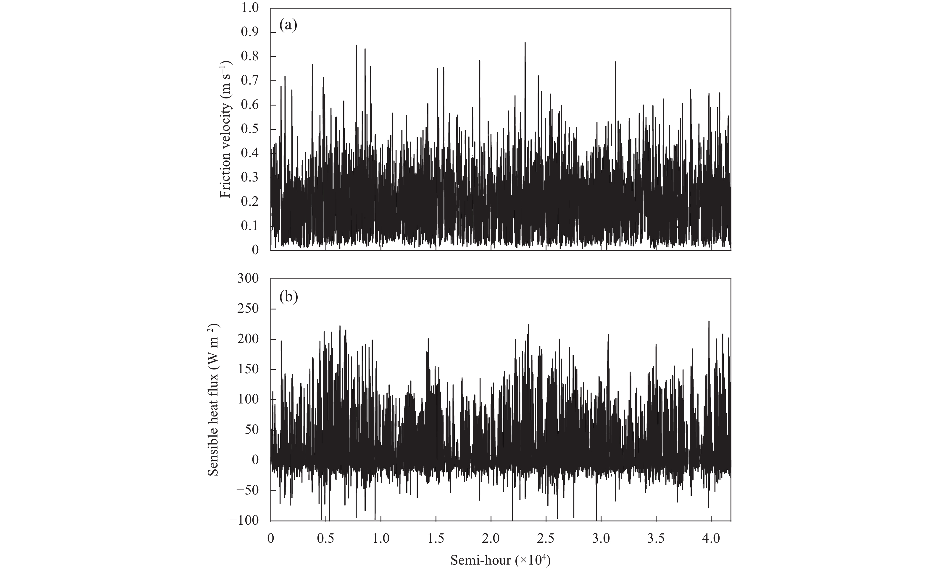
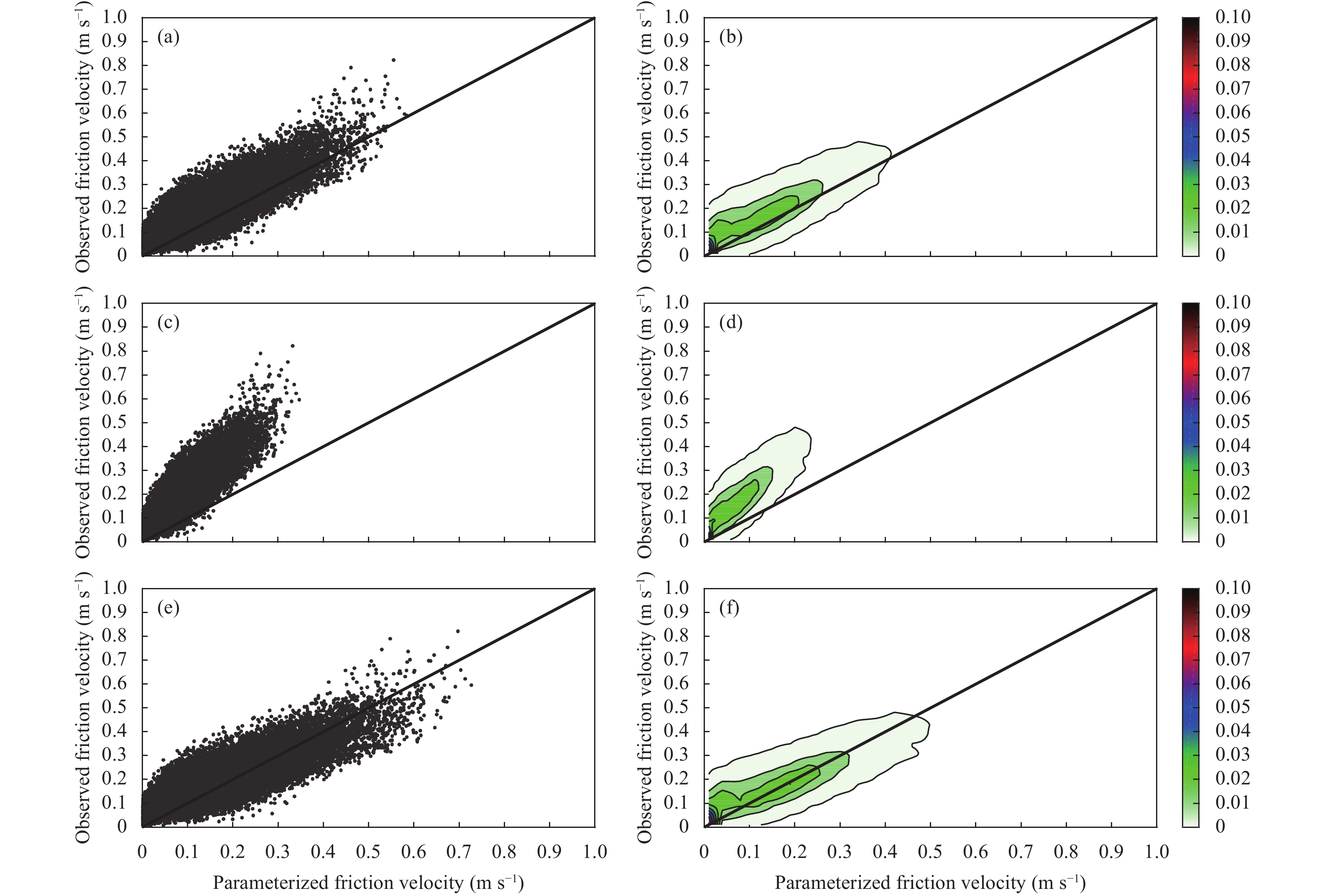
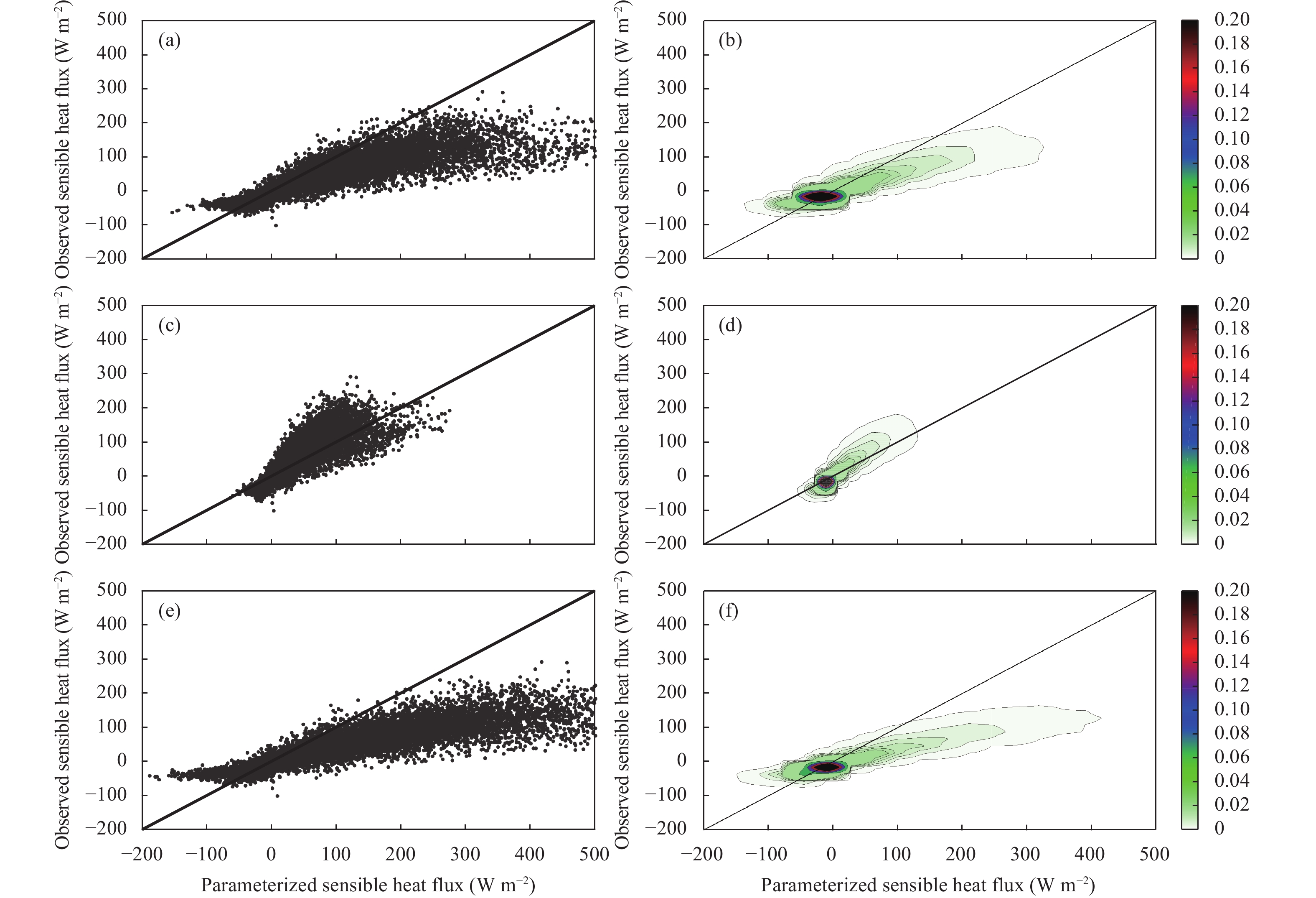
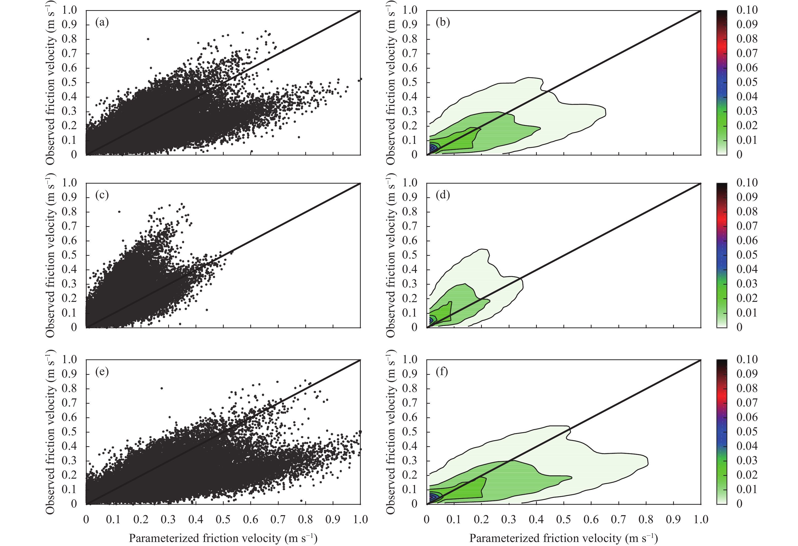
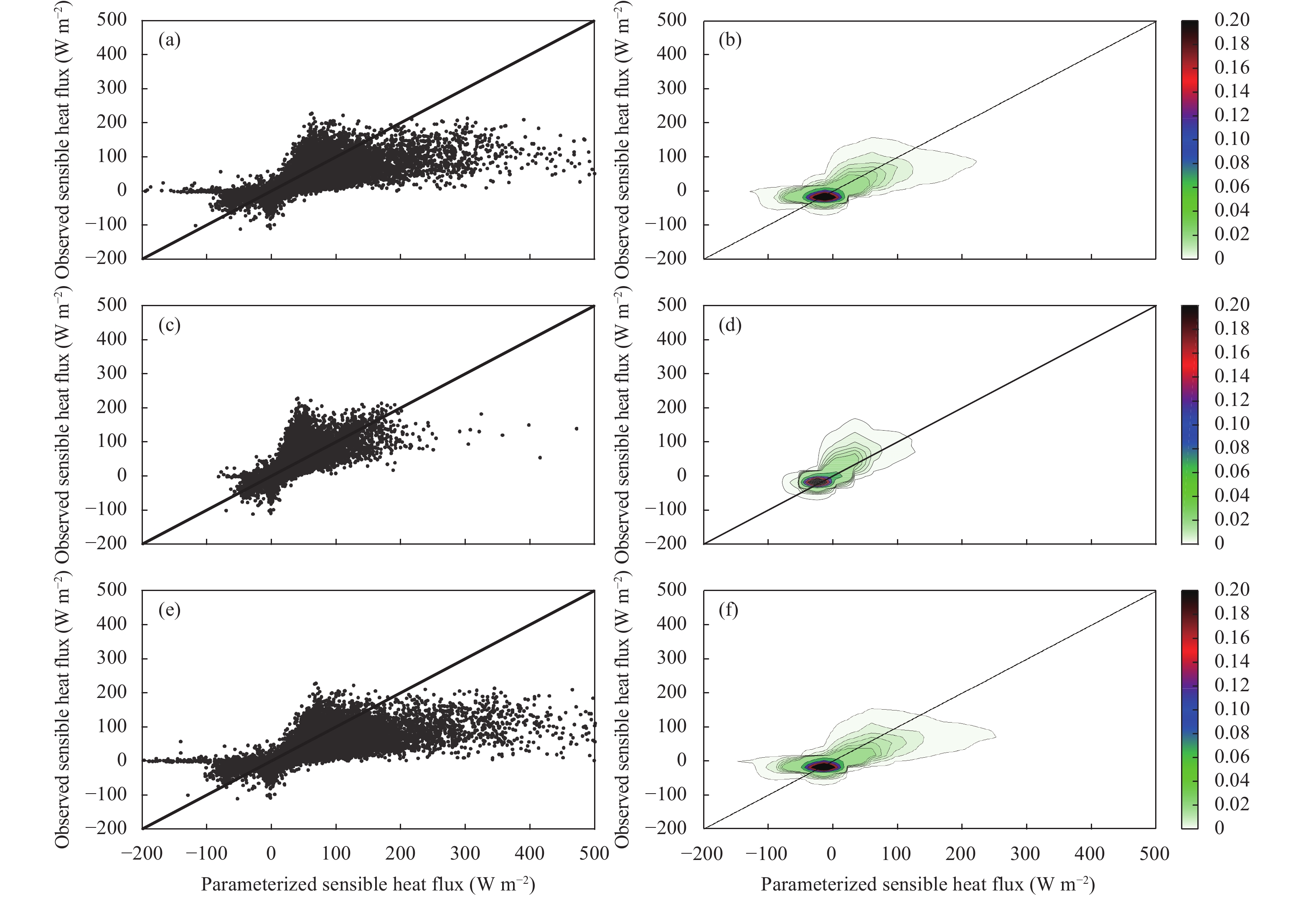
First, the turbulent statistical characteristics of the observational data are analyzed. The results shown in Table 1 indicate that the values of the fitted coefficients for turbulent statistics in the observational data are close to those suggested by Stull (1988), suggesting that the observational data follow the classical turbulent statistical law. Figures 1 and 2 show the original time series of the observed momentum and sensible heat flux at the two sites. Figures 3–10 show the comparison between the parameterized and observed surface turbulent fluxes in the form of scatter diagram and occurring probability density, and statistical quantities for the comparisons are shown in Table 2.

For the momentum flux, the parameterizations are overall in good agreement with the observations. The CAM scheme has statistical quantities similar to those that the PX scheme has at the same site, while at Jiangning, the correlation coefficients (CC) are less and the root mean square error (RMSE) and mean bias (MB) are larger than at Jiangxinzhou, indicating that the distinction in the degree of agreement between the parameterization and observation is more associated with the site than with the parameterization scheme itself. While the CC is not significantly different from one another with different ${z_0}$ , suggesting that the CC is not very sensitive to ${z_0}$ , the RMSE and MB increase with increased ${z_0}$ . In the figures, the change of the mean bias from negative to positive values with ${z_0}$ from 0.01 to 0.2 m is clearly displayed, indicating that the parameterizations underestimate the observations with ${z_0}$ = 0.01 m while overestimate them with ${z_0}$ = 0.2 m, and the parameterized momentum flux increases with increased roughness length.

For the sensible heat flux, the parameterizations in general overestimate the observations. The CAM scheme has slightly less RMSE and MB at both sites than the PX scheme, while at Jiangning, the CCs are less and the RMSE and MB are slightly less than at Jiangxinzhou, indicating the distinction in the degree of agreement between the parameterization and observation is associated with the site as well as with the parameterization scheme. While the CC is almost the same with different ${z_0}$ , the RMSE and MB increase with increased ${z_0}$ , and the sensible heat flux is overestimated except in the case of ${z_0}$ = 0.01 m where it is slightly underestimated, indicating that the parameterized sensible heat flux increases with increased roughness length.

Figures 11 and 12 are the Taylor diagrams for the comparisons between the parameterized and observed surface turbulent fluxes. In a Taylor diagram (Taylor, 2001), a dataset corresponds to a point whose coordinates are the standard deviation and correlation coefficient of the dataset. It is compared with a reference dataset (i.e., the observations in this study) that corresponds to the reference point, where the correlation coefficient of the reference dataset with itself is 1. The closer the point is to the reference point, the better the dataset is in agreement with the reference dataset statistically.

At Jiangxinzhou, for the momentum flux, the CAM and PX parameterizations reproduce the observations very well, as they have the high correlation coefficients around or above 0.8 and the standard deviations close to the observations. With ${z_0}$ = 0.01 m, the parameterizations correlate with the observations very well but underestimate the standard deviation of the observations, while the correlation is weaker and the standard deviation of the observations is overestimated with ${z_0}$ = 0.2 m. Overall, their distances from the reference point are farther, indicating that the parameterizations with seasonally-varying ${z_0}$ reproduce the observations better. For the sensible heat flux, the parameterizations correlate with the observations very well. With ${z_0}$ = 0.2 m and varying seasonally, the parameterizations overestimate the standard deviation of the observations. Although with ${z_0}$ = 0.01 m, the parameterizations underestimate the standard deviation of the observations but are comparatively closer to the observations, indicating that the parameterizations with ${z_0}$ = 0.01 m reproduce the observations relatively better.

At Jiangning, the comparisons are generally the same. However, due to decreased correlation coefficients, the parameterized datasets are relatively farther from the reference point, indicating that the parameterizations do not reproduce the observations as well as at Jiangxinzhou.

Figure 13 shows the comparison of the relative Euclidean distance for the momentum and sensible heat flux. The relative Euclidean distance $D$ is defined as (Wu et al., 2012; Liu et al., 2013)

$D = \sqrt {\;{{\left({\frac{{\bar x - \bar y}}{{\bar y}}} \right)}^2} + {{\left({\frac{{{\sigma _x} - {\sigma _y}}}{{{\sigma _y}}}} \right)}^2} + {{\left({{c_{xy}} - 1} \right)}^2}} ,$

(13)

where $x$ and $y$ denote the parameterization and observation, respectively; $\bar x$ , $\bar y$ , ${\sigma _x}$ , and ${\sigma _y}$ are the corresponding mean values and standard deviations; ${c_{xy}}$ is the correlation coefficient between $x$ and $y$ . Therefore, the value of $D$ is equal to 0 for perfect agreement and increases as the agreement degrades.

According to the relative Euclidean distances, the momentum flux parameterization performs better than the sensible heat flux parameterization. While at the same site, the two parameterizations have roughly equivalent performances, and both of them perform better at Jiangxinzhou than at Jiangning. For the friction velocity, the parameterizations with seasonally-varying ${z_0}$ have better performance, while for the sensible heat flux, the parameterizations with ${z_0}$ = 0.01 m perform relatively better.

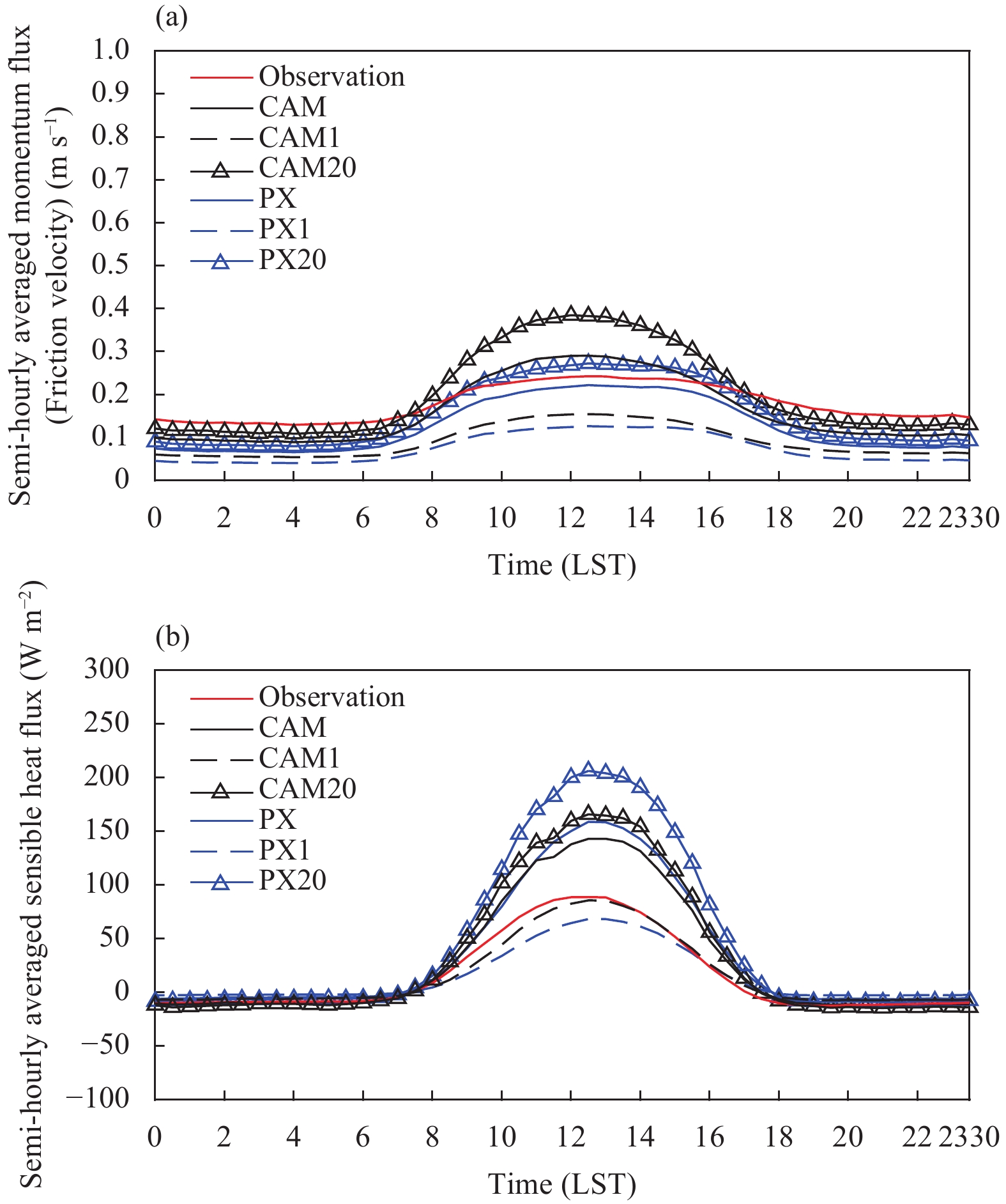
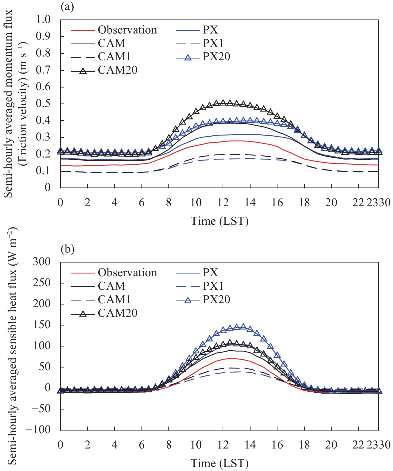
Figures 14 and 15 compare the diurnal pattern between the parameterized and observed surface turbulent flux. Both of the parameterizations capture the diurnal pattern seen in the observations at the two sites very well, but the parameterizations overestimate the sensible heat flux in the daytime at the sites except the two cases with the lower limit of ${z_0}$ , which slightly underestimate them in the daytime. At Jiangxinzhou, the CAM parameterization overestimates the momentum flux around the noon and the PX parameterization underestimates it throughout the day, while both of the parameterizations overestimate the momentum flux throughout the day at Jiangning, suggesting that overall the two parameterizations reproduce relatively larger momentum fluxes at Jiangning than at Jiangxinzhou. However, the difference between the two parameterizations in reproducing the momentum and sensible heat flux is not significant in terms of the statistical quantities shown in Table 2. In addition, the larger the roughness length is, the larger the parameterized flux is.

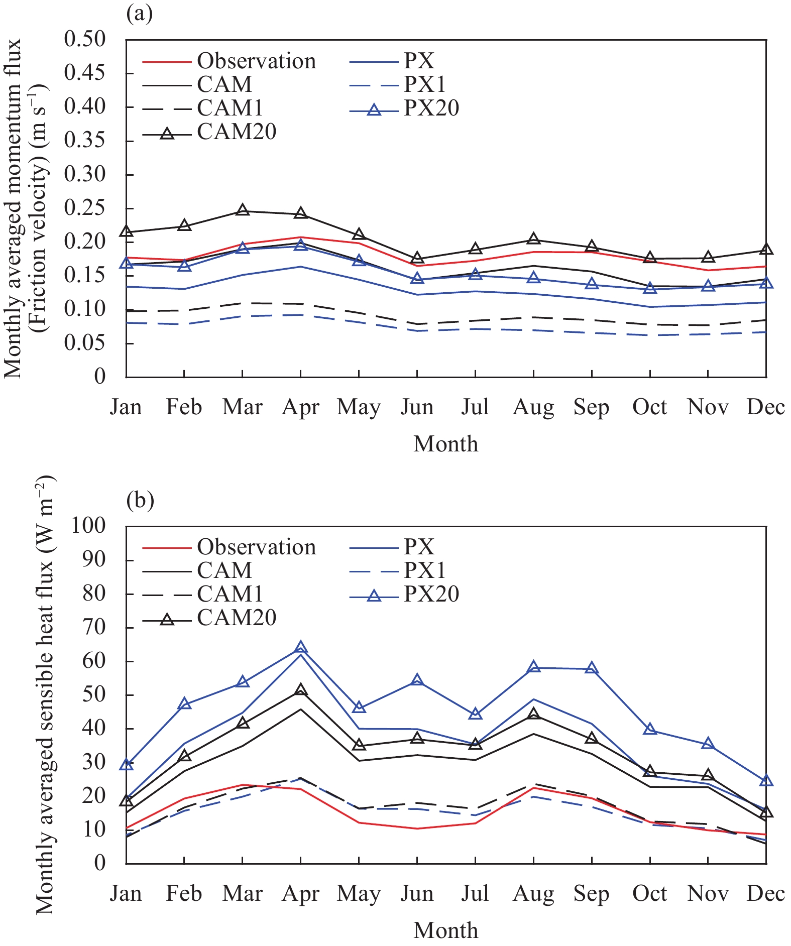
Figures 16 and 17 compare the seasonal pattern between the parameterized and observed surface turbulent flux. Both of the parameterizations capture the seasonal pattern seen in the observations at the two sites well. While over the entire year the momentum flux is slightly underestimated at Jiangxinzhou and slightly overestimated at Jiangning in terms of statistics, the sensible heat flux is overestimated at both Jiangxinzhou and Jiangning. Moreover, the parameterized sensible heat flux is larger in the spring and late summer at Jiangxinzhou and in the late summer and autumn at Jiangning. While the cause warrants further investigation and study, we infer that it may be due to larger land–air temperature difference at those times of the year. In addition, the overall difference between the parameterizations is not significant, and the parametrized fluxes increase with increased ${z_0}$ .

5 Conclusions and discussion

Field measurements of the turbulent momentum and sensible heat flux in the surface layer were conducted over homogenous and flat grassland in two meteorological observing yards in the suburb of Nanjing, eastern China for longer than 2 yr. The variances of the turbulent observational data display consistent statistical characteristics, and the values of fitted coefficients are close to those suggested by Stull (1997). The flux observational data are then used to evaluate the CAM and PX parameterization schemes reproducing the turbulent momentum and sensible heat flux in the surface layer. It is found that the momentum flux parameterizations are in good agreement with the observations, while the sensible heat flux parameterizations overestimate the observations, which is in coincidence with previous research (Liu et al., 2013, 2017).

Overall, the momentum flux parameterizations reproduce the observations very well in terms of the root mean square error and mean bias. In the Taylor diagram, compared to the sensible heat flux parameterizations, the momentum flux parameterizations are close to the observations, as the centered root mean square error (i.e., the distance between the parameterization and observation point) for the momentum flux is less, indicating that the momentum flux is better reproduced than the sensible heat flux. The relative Euclidean distance between the parameterization and observation for the momentum flux is less than that for the sensible heat flux. The momentum flux parameterizations capture the diurnal and seasonal patterns seen in the observations very well. While the momentum flux is underestimated at Jiangxinzhou in terms of seasonal pattern, the sensible heat flux is overestimated at Jiangning in terms of both diurnal and seasonal patterns.

The sensible heat flux parameterizations systematically overestimate the observations in terms of the root mean square error and mean bias. In the Taylor diagram, the distance between the parameterization and observation point is farther, and the relative Euclidean distance between the parameterization and observation is larger, indicating that the reproduction of the observations by the parameterizations for the sensible heat flux is not so good as for the momentum flux. The parameterizations also capture the diurnal and seasonal patterns seen in the observations well, but the parameterizations overestimate the observations in the daytime in diurnal pattern and over the entire year in seasonal pattern. The results are also in coincidence with previous research (Liu et al., 2013, 2017).

It should be kept in mind that the correlation between the observation and parameterization is overall high due to the nature of the data in this study. Since the observed ground temperature that drives the sensible heat flux and the observed wind speed that drives the friction velocity are driven by the solar cycle and increase and decrease predictably over the diurnal cycle, the parameterized fluxes do as well, and the correlation between the observation and parameterization is predictably high. Therefore, most focus should be on the RMSE and MB.

One of the causes why the momentum flux parameterization performs better than the sensible heat flux parameterization could be the difference of temperature between the land and atmosphere (Liu et al., 2013, 2017). Theoretically, the surface air temperature, which is the air temperature at the height of the thermal roughness length z_0h, should be used. However, due to the difficulty of determining z_0h accurately at present, the surface air temperature is hard to measure as well as to calculate; in reality, the ground temperature is used for the replacement of the surface air temperature. While the surface air temperature is not needed in the parameterization of the momentum flux, this reduces the error between the parameterized and observed momentum flux compared to the sensible heat flux.

In general, the difference between the parameterizations in reproducing the momentum and sensible heat flux is not significant in terms of statistical quantities. This conclusion should be reasonable and expected, since the parameterizations are constructed on the common framework of theory (i.e., the Monin–Obukhov Similarity Theory). Overall, the parameterizations perform better at Jiangxinzhou than at Jiangning in terms of the correlation coefficient, of which the reason is to be explored in further analysis.

Checking the effect of the roughness length ${z_0}$ on the parameterization indicates that the parameterized fluxes increase with increased ${z_0}$ . That is to say, when the parameterization with smaller ${z_0}$ underestimates the flux, the parameterization with larger ${z_0}$ may reproduce the flux better. However, when the parameterization with smaller ${z_0}$ already overestimates the flux, the parameterization with larger ${z_0}$ may overestimate the flux further, and vice versa.

In general, improving the performance of a flux parameterization scheme has to involve with many factors (Liu et al., 2013, 2017). This evaluation suggests that among many factors that could contribute to improvement of a scheme of surface turbulent flux parameterization, how to determine the surface air temperature and improve the common theoretical framework of the Monin–Obukhov Similarity Theory may stand out, although some progresses have been made in recent years, especially on the applicability of the Monin–Obukhov Similarity Theory under stable conditions (e.g.,Chenge and Brutsaert, 2005; Grachev et al., 2007; Sharan and Kumar, 2011; Li et al., 2014). In addition, since this evaluation is conducted against field observational data in eastern China, it also provides a practical knowledge of the comparison between the fluxes estimated by the surface layer parameterization schemes and those measured by in-situ observations and is helpful in understanding the performance of the parameterizations in the region.

Acknowledgments. The authors declare that there is no conflict of interest regarding the publication of this paper. The authors thank the anonymous reviewers for their constructive criticism and comments, which have greatly helped to improve the quality of this study.