The Chinese Meteorological Society
Article Information
- LIU, Yongzhu, Lin ZHANG, and Zhihua LIAN, 2018.
- Conjugate Gradient Algorithm in the Four-Dimensional Variational Data Assimilation System in GRAPES. 2018.
- J. Meteor. Res., 32(6): 974-984
- http://dx.doi.org/10.1007/s13351-018-8053-2
Article History
- Received April 8, 2018
- in final form August 20, 2018
The application of high-resolution data assimilation constitutes a mainstream technology for improving numerical weather prediction (NWP) models. Variational data assimilation, which is used to solve analysis problems by minimizing a given cost function, is the best way to estimate model initial conditions by accurately combining observation and background fields (Rabier, 2005; Bannister, 2017). Three-dimensional variational data assimilation (3DVar) was widely used in NWP centers during the twentieth century (Courtier et al., 1998; Rabier et al., 1998; Lorenc et al., 2000). However, 3DVar erroneously assumes that observations acquired at different times are taken at the same time within the assimilation window. To overcome the shortcomings of 3DVar, four-dimensional variational data assimilation (4DVar) seeks an optimal balance between observations scattered through time and space over a finite 4D analysis volume with priori information; consequently, 4DVar is able to closely fit both observations and a priori initial estimates to generate the optimal initial conditions for NWP models (Thépaut et al, 1993; Courtier et al., 1994). For more than a decade, 4DVar has been the most successful data assimilation method for global NWP models; it has been used by many of the main global NWP centers, such as the ECMWF (Rabier et al., 2000), the French national meteorological service Météo-France (Janisková et al., 1999), the Met Office (Rawlins et al., 2007), and the meteorological service of Canada (Laroche et al., 2007). In recent years, some new 4DVar methods for global NWP models have emerged, including the ensemble-based 4DVar technique (Liu and Xiao, 2013) and hybrid 4DVar that adds flow-dependent ensemble covariance to traditional incremental 4DVar, for example, the ensemble data assimilations at ECMWF (Isaksen et al., 2010) and the hybrid-4DVar method employed at the Met Office (Clayton et al. 2013;Lorenc et al., 2015).
Variational data assimilation is a solution to large-scale unconstrained optimization problems. The cost function measuring the misfit between the background and the observations is first defined, and the optimal values are then determined by using various large-scale unconstrained minimization algorithms. Variational data assimilation techniques, especially 4DVar approaches based on the tangent linear model and adjoint model, are computationally expensive; thus, the development of a robust and efficient minimization algorithm is crucial (Fisher, 1998; Gürol et al., 2014). Two common minimization algorithms used in 4DVar systems are the conjugate gradient algorithm (CGA; Fisher, 1998) and quasi-Newton methods, including the limited-memory quasi-Newton method (i.e., the limited-memory Broyden–Fletcher–Goldfarb–Shanno, L-BFGS; Liu and Nocedal, 1989) and the truncated Newton method (Nash, 1984). Just as the L-BFGS method attempts to combine the modest storage and computational requirements of CGA methods with the convergence properties of standard quasi-Newton methods, truncated Newton methods attempt to retain the rapid (quadratic) convergence rate of classic Newton methods while making the storage and computational requirements feasible for large sparse matrices (Zou et al., 1993). Zou et al. (1993) compared the L-BFGS method with two truncated Newton methods on several test problems, including problems in meteorology and oceanography; their results confirmed that the L-BFGS seems to be the most efficient approach and is a particularly robust and user-friendly technique. Navon and Legler (1987) compared a number of different CGA and L-BFGS approaches for problems in meteorology and concluded that the L-BFGS is the most adequate for large-scale unconstrained minimization algorithms in meteorology. Furthermore, Fisher (1998) compared different CGA and truncated Newton methods in the ECMWF, and they concluded that the CGA was the most adequate for their 4DVar system. Therefore, the preconditioned CGA is used in the operational 4DVar system of ECMWF (Trémolet, 2007).
The 3DVar operational assimilation system is employed in the Global/Regional Assimilation and Prediction System (GRAPES; Shen et al., 2017) with the L-BFGS minimization algorithm (Xue et al., 2008). The GRAPES dynamical core uses a non-hydrostatic framework with two-time-layer semi-implicit and semi-Lagrangian discretization and employs a latitude–longitude grid with the staggered Arakawa C grid for spatial discretization. A 4DVar system has been developed in the GRAPES to improve its operational prediction quality by using the non-hydrostatic tangent linear and adjoint models, which were developed for the GRAPES global data assimilation system (Liu et al., 2017). The L-BFGS method is currently applied to the GRAPES 4DVar system, but its low convergence rate leads to a low computational efficiency (Zhang and Liu, 2017). In this paper, to select a robust and efficient minimization algorithm for the GRAPES 4DVar system, the convergence of the CGA is thoroughly examined, and the CGA is compared with the L-BFGS method in the GRAPES 4DVar scheme.
This paper is organized as follows. The data and methods are described in Section 2. Section 3 investigates the convergence of the CGA, and some results of the CGA in the GRAPES 4DVar system based on the numerical experiments are presented in Section 4. The conclusions and outlook are presented in Section 5.
2 Data and methods 2.1 Incremental 4DVarIncremental formulation is commonly used in variational data assimilation systems (Courtier et al., 1994; Trémolet, 2007). The incremental scheme offers two main advantages: 1) the tangent linear model and adjoint model can be used with a reduced resolution during minimization, largely reducing the computational cost of 4DVar; 2) the cost function becomes strictly quadratic, and thus, the convergence rate of the minimization can be greatly improved (Fisher, 1998). The incremental formulation scheme includes two components, namely, the inner loop and the outer loop. The outer loop utilizes the initial estimate of the atmospheric state as the initial condition of the forecast model and obtains the model trajectory within the assimilation time windows; this trajectory is then used to calculate the observational increments within the time windows. The purpose of the inner loop is to solve the minimization problem by an iterative algorithm for the variational data assimilation.
In the 4DVar incremental formulation, the first-order approximation of the cost function
| $\begin{split} J \left( {\delta {x}} \right) & = \frac{1}{2}\delta {{x}^{\rm{T}}}{{{B}}^{{ - 1}}}\delta {x} + \frac{1}{2}{\sum\nolimits_{{i} = 0}^{n} {\left( {{{{H}}_{i} }{{{L}}_{0 \to {i}}}\delta {x} - {{d}_{i}}} \right)} ^{\rm{T}}}{{R}}_{i}^{{ - 1}}\left( {{{{H}}_{i} }{{{L}}_{0 \to {i}}}\delta {x} - {{d}_{i}}} \right) \\& =\frac{1}{2}\delta {{x}^{\rm{T}}}\left( {{{{B}}^{ - 1}} + \sum\nolimits_{{i} = 0}^{n} {{{L}}_{{i} \to 0}^{\rm{T}}{{H}}_{i}^{\rm{T}}{{R}}_{i}^{{ - 1}}{{{H}}_{i}}{{{L}}_{0 \to {i}}}} } \right)\delta {x} - \delta {{x}^{\rm{T}}}\sum\nolimits_{{i} = 0}^{n} {{{L}}_{{i} \to 0}^{\rm{T}}{{H}}_{i}^{\rm{T}}{{R}}_{i}^{{ - 1}}{{d}_{i}}} + \frac{1}{2}{d}_{i}^{\rm{T}}{{R}}_{i}^{{ - 1}}{{d}_{i}}\end{split},$ | (1) |
where
To solve the minimization problem of Eq. (1), the gradient of the control variable δx is calculated with the following equation (Courtier et al., 1994; Fisher, 1998):
| $\begin{split}\nabla {J}\left({\delta {x}} \right) = & \left({{{{B}}^{ - 1}} + \sum\nolimits_{{i} = 0}^{n} {{{L}}_{{i} \to 0}^{\rm{T}}{{H}}_{i}^{\rm{T}}{{R}}_{i}^{ - 1}{{{H}}_{i}}{{{L}}_{0 \to {i}}}} } \right)\delta {x} \\ - & \sum\nolimits_{{i} = 0}^{n} {{{L}}_{{i} \to 0}^{\rm{T}}{{H}}_{i}^{\rm{T}}{{R}}_{i}^{ - 1}{{d}_{i}}}, \end{split}$ | (2) |
where the minimization of the cost function can be obtained by minimization algorithms such as the Newton method or CGA. The second partial derivative of
| ${J''} = {{{B}}^{ - 1}} + \sum\nolimits_{{i} = 0}^{n} {{{L}}_{{i} \to 0}^{\rm{T}}{{H}}_{i}^{\rm{T}}{{R}}_{i}^{ - 1}{{{H}}_{i}}{{{L}}_{0 \to {i}}}} .$ | (3) |
Thus, the solution of Eq. (2) is equal to the solution of the system of linear equations
Because B is usually a large sparse matrix and is nearly ill conditioned, it is difficult to solve the minimization problem in Eq. (1). To achieve acceptable convergence rates, it is necessary to perform some transforms and preconditioning for B.
In the GRAPES 4DVar system, the basic atmospheric state variables x are the two wind vectors (denoted by u and v), the relative humidity q, and the non-dimensional pressure as an independent variable (denoted by
Therefore, the background error covariance matrix B can be split into three independent blocked matrices
| $\begin{split}J\left({w} \right) = & \frac{1}{2}{{w}^{\rm{T}}}{w} + \frac{1}{2}{\sum\nolimits_{{i} = 0}^{n} {\left({{{{H}}_{i} }{{{L}}_{0 \to {i}}}\mathcal{P}{\Sigma _{u}}\mathbb{U}{w} - {{d}_{i}}} \right)} ^{\rm{T}}}\\ & \cdot {{R}}_{i}^{ - 1}\left({{{{H}}_{i} }{{{L}}_{0 \to {i}}}\mathcal{P}{\Sigma _{u}}\mathbb{U}{w} - {{d}_{i}}} \right).\end{split}$ | (4) |
The L-BFGS algorithm (Appendix A) in the GRAPES 4DVar system uses the estimation to the inverse Hessian matrix to guide its search through the variable space. For the L-BFGS in the GRAPES 4DVar scheme, the initial Hessian matrix is the identity matrix, and the number of iterations m insomuch that the m previous values sk and zk are stored to compute the approximation of the inverse Hessian matrix is 12.
The CGA based on the Lanczos iteration (Appendix B) in GRAPES 4DVar is mainly applied to solve large sparse, symmetric, positive definite linear equations (Paige and Saunders, 1982). With this combination, the orthogonalization of the Lanczos algorithm can sufficiently overcome the instability of the CGA in providing practical solutions to the above equations.
The Hessian matrix
Rounding errors greatly affect the behavior of the Lanczos iteration for a practical minimization problem (Paige, 1970). For a 4DVar system in particular, there are often some computational errors from the tangent model and adjoint model of the Hessian matrix
(1) Full orthogonalization (Paige, 1970). This process conducts Gram-Schmidt orthogonalization to make the Lanczos vector
(2) Partial orthogonalization (Simon, 1984). Consequently, instead of orthogonalizing
(3) Selective orthogonalization (Parlett and Scott, 1979). The method is similar to partial orthogonalization but orthogonalizing
The CGA has been successfully applied in the 4DVar system of ECMWF (Fisher, 1998; Trémolet, 2007). However, there are many differences between the GRAPES and ECMWF 4DVar systems. First, the ECMWF tangent linear model and adjoint model use a hydrostatic framework with spectral and reduced grids, while those in GRAPES employ a non-hydrostatic framework with a latitude–longitude grid. Especially in polar regions, the denser grid distribution of GRAPES adds a gradient sensitivity computed by the adjoint model, leading to an increase in the condition number of the Hessian matrix
To further analyze the effectiveness of the CGA in a practical 4DVar system, we conduct one cycling assimilation experiment for a month. The time ranges from 0900 UTC 1 June to 0900 UTC 1 July 2016. The data used for the assimilation include conventional Global Telecommunication System (GTS) observations, including temperature, wind and relative humidity data derived from sounding, pressure data from ships and the Synoptic Ocean Prediction (SYNOP) experiment, and wind data from pilot readings, in addition to data from satellite-based platforms, such as the NOAA-15 Advanced Microwave Sounding Unit-A (AMSUA), NOAA-18 AMSUA, NOAA-19 AMSUA, MetOp-A AMSUA, MetOp-B AMSUA, National Polar-orbiting Partnership (NPP) Advanced Technology Microwave Sounder (ATMS) AMSUA, SeaWinds scatterometer, and Global Navigation Satellite System (GNSS) radio occultations. Satellite observations compose approximately 70% of the total observations. The assimilation window is 6 h, and the observational interval is 30 min. The horizontal resolution of the outer loop is 0.5°, and the model time step is 450 s. The horizontal resolution of the inner loop is 1.5°, and the model time step is 900 s. The number of vertical levels is 60, and the maximum number of iterations is 70 in the 4DVar minimization.
The following linearized physical processes are used in this 4DVar experiment: two dry linearized physical processes (vertical diffusion and subgrid-scale orographic effects) to improve the representation of perturbed fields in the tangent linear model (Liu et al., 2017), and two newly developed moist linearized physical parameterizations consisting of deep cumulus convection based on a new simplified Arakawa-Shubert scheme (Han and Pan, 2006) and the large-scale cloud and precipitation scheme described in Tompkins and Janisková (2004). The experimental environment is based on the high-performance computer (Sugon PI) at the China Meteorological Administration. In total, 256 CPU cores are used in these experiments. Two configurations of 4DVar experiments are tested:
(1) CGA experiments, in which the CGA is used for minimization in the 4DVar system; and
(2) L-BFGS experiments, in which the L-BFGS is used for minimization in the 4DVar.
4 Results of the CGA in 4DVarWe perform numerical experiments on the GRAPES 4DVar system to investigate the convergence of the CGA therein. The experimental configuration is the same as that in the batch experiments in Section 3, which begin at 0900 UTC 1 June 2016, and the number of iterations is 120 in the minimization. Then, the numerical stability of the Lanczos algorithm in the 4DVar is tested against the four orthogonalization schemes described in Section 2.3: full orthogonalization, partial orthogonalization, selective orthogonalization, and without orthogonalization.
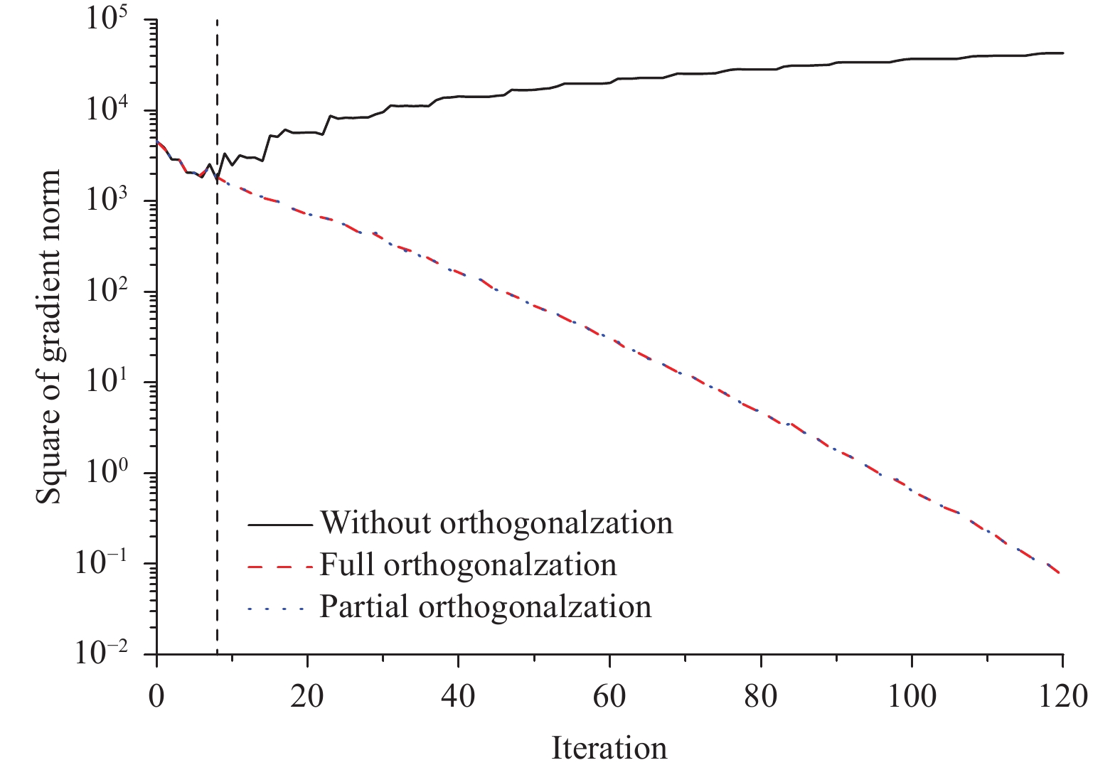
4.1 Orthogonalization analysis of the CGAThe convergence of the gradient norm
|
| Figure 1 Convergence of the conjugate gradient norm as a function of the number of iterations for a 4DVar cost function. The vertical axis is the square of the gradient norm, and it denotes the difference between the control vector at a given iteration and its 120th iteration (black solid line: without orthogonalization; red dashed line: full orthogonalization; blue dotted line: partial orthogonalization; vertical dotted line shows that the gradient norm fails to converge starting at the 9th iteration without orthogonalization). |
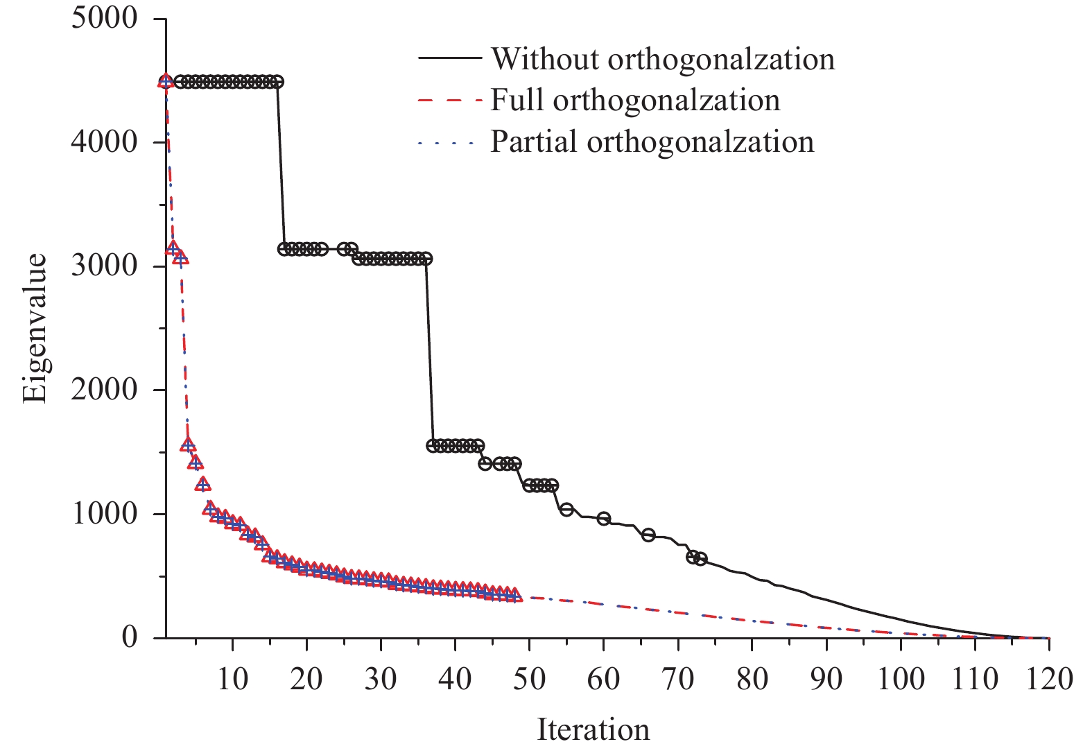
The eigenvalue distribution of the Hessian matrix
|
| Figure 2 Eigenvalue distribution of the Hessian matrix of a 4DVar minimization with different schemes of the orthogonalization of Lanczos vectors against the number of iterations (black solid line: without orthogonalization; red dashed line: full orthogonalization; blue dotted line: partial orthogonalization). |
In the 4DVar minimization, the convergence rate of the CGA depends on the eigenvalue distribution of the Hessian matrix
| $\left\| {{{e}_{j}}} \right\|_{{J''}}^2 \!=\! {\left({\delta {x} \!-\! \delta {{x}_{j}}} \right)^{\rm{T}}}{J''}\left({\delta {x} \!-\! \delta {{x}_{j}}} \right) \leqslant 2{\left({\frac{{\sqrt {\kappa } \!-\! 1}}{{\sqrt {\kappa } \!+\! 1}}} \right)^{j}}\left\| {{{e}_{0}}} \right\|_{{J''}}^2.$ | (5) |
Here, δx is the solution of the 4DVar minimization in Eq. (1) (the value of which is the estimated solution of the last iteration of the CGA), while
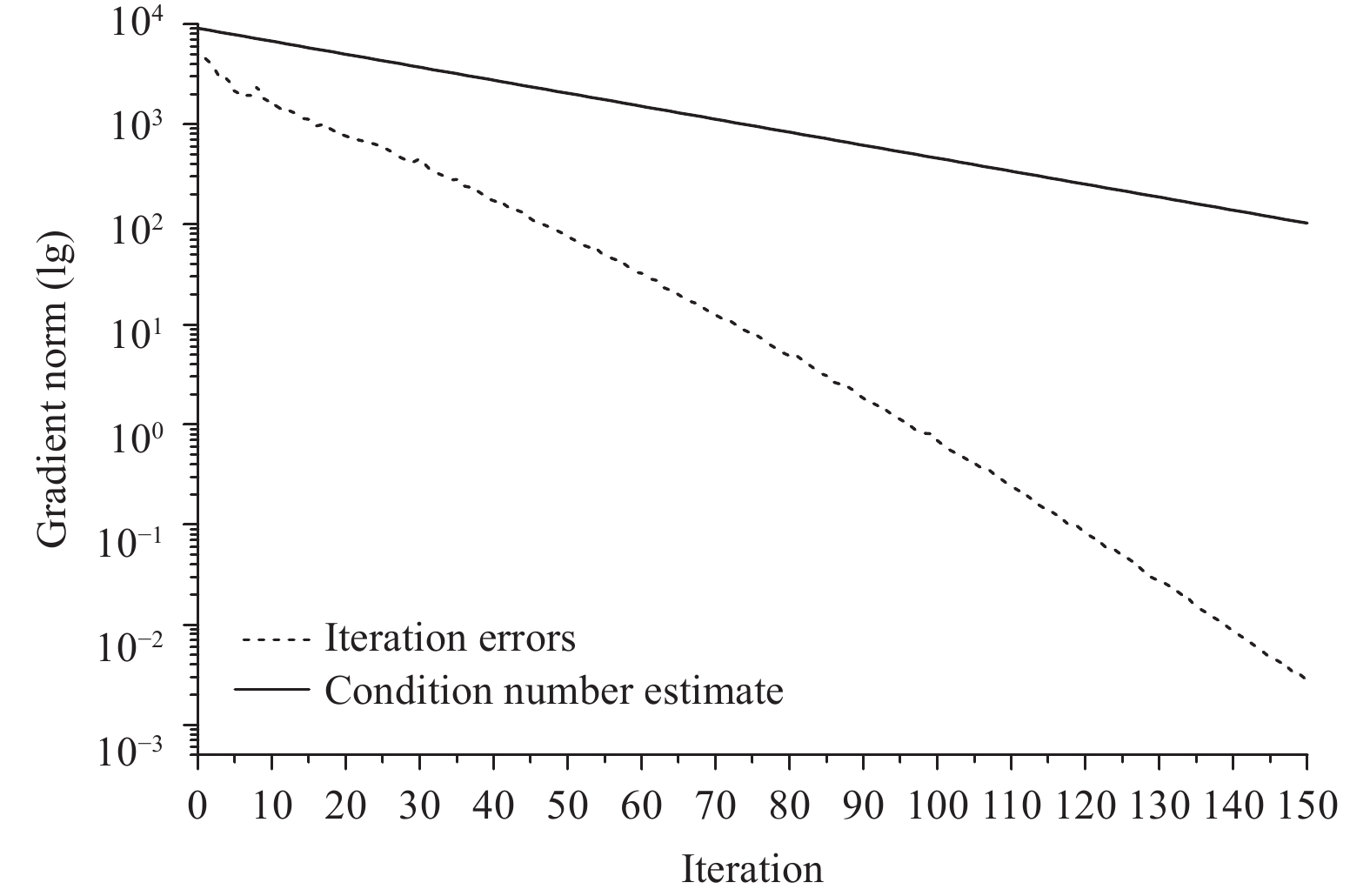
To explore the convergence of the CGA in the GRAPES 4DVar system, we conduct an assimilation experiment (beginning at 0900 UTC 1 June 2016) with 120 iterations of 4DVar minimization. The maximum (minimum) eigenvalue of the Hessian matrix
|
| Figure 3 Convergence of the CGA as a function of the number iterations for a 4DVar cost function. The dashed line is the square of the Hessian norm of the difference between the control vector and the value of the last iteration. The solid line is the upper bound of the convergence rate defined by Eq. (5). |
In short, the Lanczos algorithm is numerically more stable in the 4DVar minimization if the Lanczos vector is orthogonal during the Lanczos iterations. Thus, performing Gram-Schmidt orthogonalization on the Lanczos vector is an effective way to ensure the numerical stability in the Lanczos algorithm. In this way, the convergence rate of 4DVar minimization is also improved. Considering the short computational time for orthogonalization in the whole 4DVar system, we exploit the Lanczos algorithm with full orthogonalization in the GRAPES 4DVar system to guarantee the orthogonality of the Lanczos vector.
5 Results of numerical experiments in 4DVar 5.1 Comparison of convergence with the L-BFGSThe CGA and quasi-Newton method are both quadratically convergent in theory and have the same quadratic termination property. However, these methods behave quite differently in practical applications, especially when applied to certain problems such as solving the minimization of 4DVar. To better compare the convergences of these two methods in 4DVar minimization problems, both cycling assimilation experiments begin on 10 June 2016. Recalculations are performed in the 4DVar experiments with the CGA using the background from the L-BFGS tests. The ratio of the root mean square of the gradient norm to its initial value is regarded as the convergence criterion (set as 0.03) during the minimization iterations. The maximum number of iterations is 70.
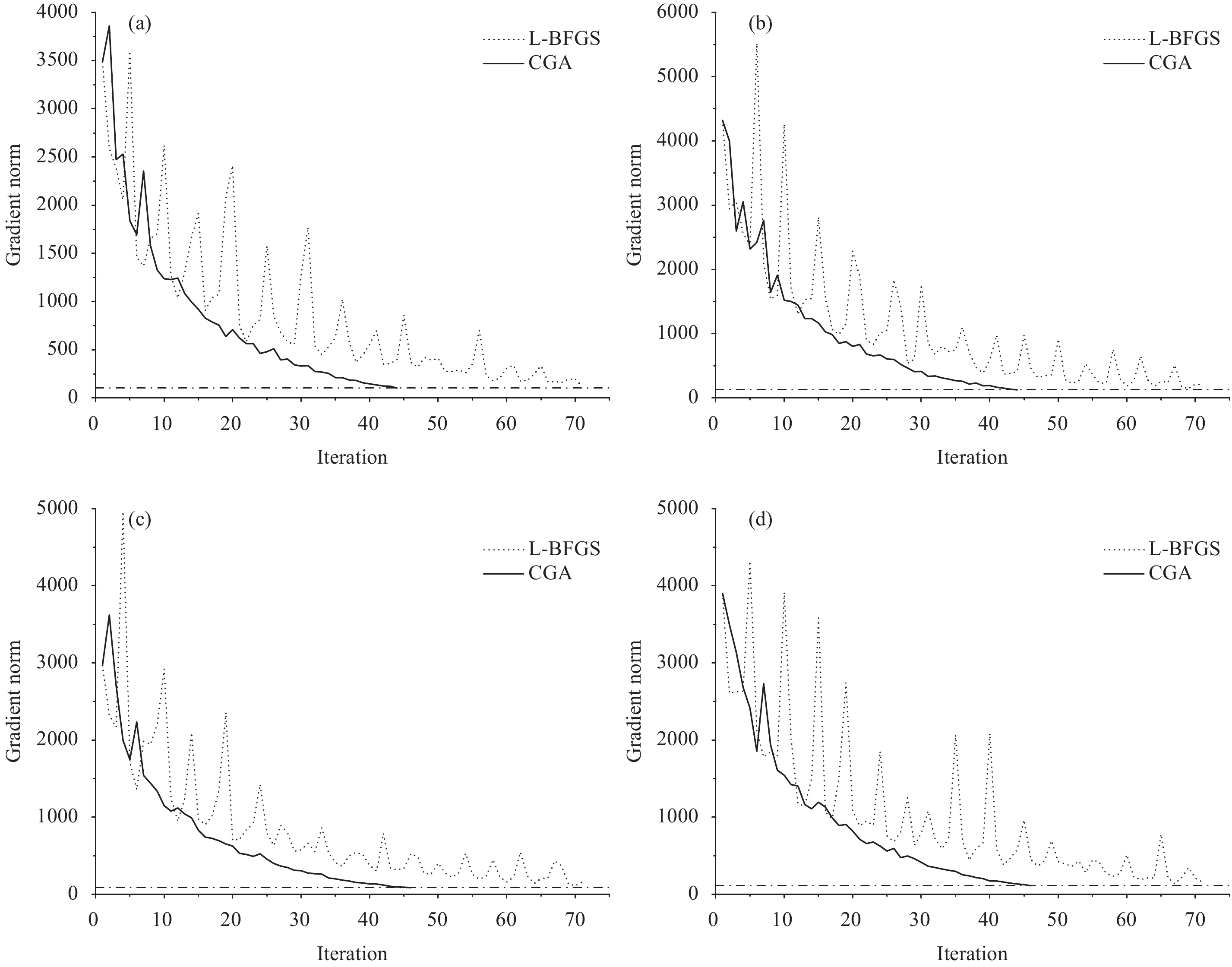
In the first dozen 4DVar minimization iterations in the four assimilation experiments, the gradient norms of the CGA and L-BFGS experiments both decrease with some oscillations, and a smaller amplitude is observed for the CGA experiments (Fig. 4). Then, the oscillation of the gradient norm for the CGA experiments becomes small, and these experiments satisfy the convergence criterion after approximately 40 iterations. However, the oscillation of the gradient norm for the L-BFGS experiments is still large, and the experiments do not converge after 70 iterations. In addition, the gradient norm in the L-BFGS experiments descends very slowly in the later stages, and the minimum is similar to that after approximately 40 iterations in the CGA experiments (dotted line in Fig. 4). The above results indicate that the convergence of the CGA is better than that of the L-BFGS in the 4DVar minimization. Moreover, the computational cost of the CGA is lower. Therefore, the CGA is preferable.
|
| Figure 4 Convergence of the Hessian norm for a 4DVar cost function under the GRAPES global 4DVar assimilation system starting at (a) 0300 UTC 10 June 2016, (b) 0900 UTC 10 June 2016, (c)1500 UTC 10 June 2016, and (d) 2100 UTC 10 June 2016 (solid line: CGA experiment; dotted line: L-BFGS experiment). |
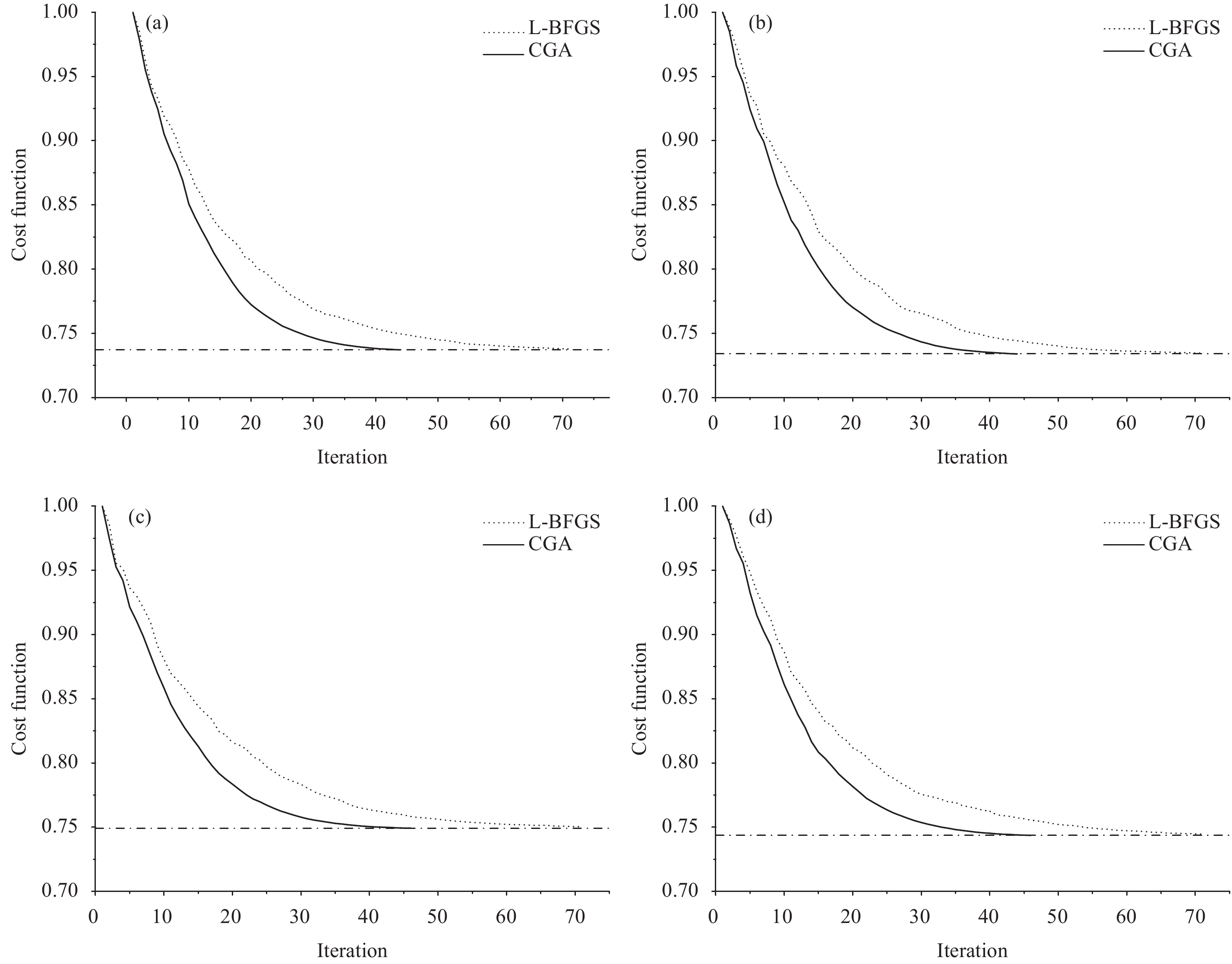
To better compare the convergences of the cost functions between the two sets of experiments, normalization is applied to the cost function to calculate the ratio of all the cost functions to the initial cost function within the iterations. The convergences of the cost functions for both the CGA experiments and the L-BFGS experiments on 20 June 2016 in the 4DVar cyclical assimilations are illustrated in Fig. 5. In the first twenty iterations, the descent rate of the cost functions of the CGA experiments are faster than those of the L-BFGS experiments. The convergence in the CGA experiments after 40 iterations is similar to that in the L-BFGS experiments after 70 iterations. Thus, the convergence rate of the CGA is much faster than that of the L-BFGS in the 4DVar minimization.
|
| Figure 5 Convergence of the 4DVar cost function under the GRAPES global 4DVar assimilation system starting at (a) 0300 UTC 20 June 2016, (b) 0900 UTC 20 June 2016, (c) 1500 UTC 20 June 2016, and (d) 2100 UTC 20 June 2016 (solid line: CGA experiment; dotted line: L-BFGS experiment; horizontal dashed line: final convergence rate of the cost function in the CGA experiment). |
In the 4DVar minimization, the term
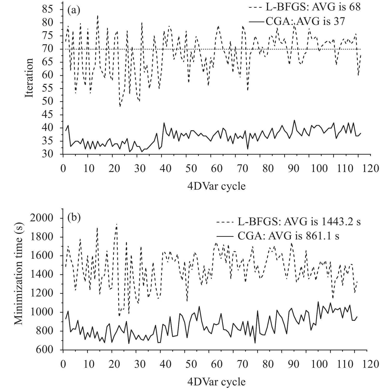
The numbers of iterations and the calculation times for the 4DVar minimization in the 121 cyclical assimilation tests for both experimental sets are plotted in Fig. 6. The CGA experiments satisfy the requirement for convergence within a maximum of 70 iterations in the minimization. The average number of iterations to reach convergence is 37, and the average minimization time in these CGA experiments is 861 s. However, most of the L-BFGS experiments do not meet this convergence requirement within the maximum number of iterations because some of the cost functions in the iterations do not decrease when using the L-BFGS minimization, and thus, it is necessary to choose another descent direction for the L-BFGS experiments, which requires additional calculations. Thus, the number of iterations for some L-BFGS experiments is greater than the maximum number of iterations (70). Furthermore, the average number of iterations in these L-BFGS experiments is 68, and the average minimization time in these L-BFGS experiments is 1443 s. The average number of iterations in the CGA experiments is 32 less than that in the L-BFGS experiments, representing a 45% improvement in the computational efficiency. Hence, the CGA can largely improve the computational efficiency without affecting the convergence in the GRAPES 4DVar system.
|
| Figure 6 (a) Number and (b) time of iterations in the 4DVar minimization in the 121 cyclical assimilation tests for the two experimental sets (solid line: CGA experiment; dashed line: L-BFGS experiment; AVG: the average number or time of iterations over one month) |
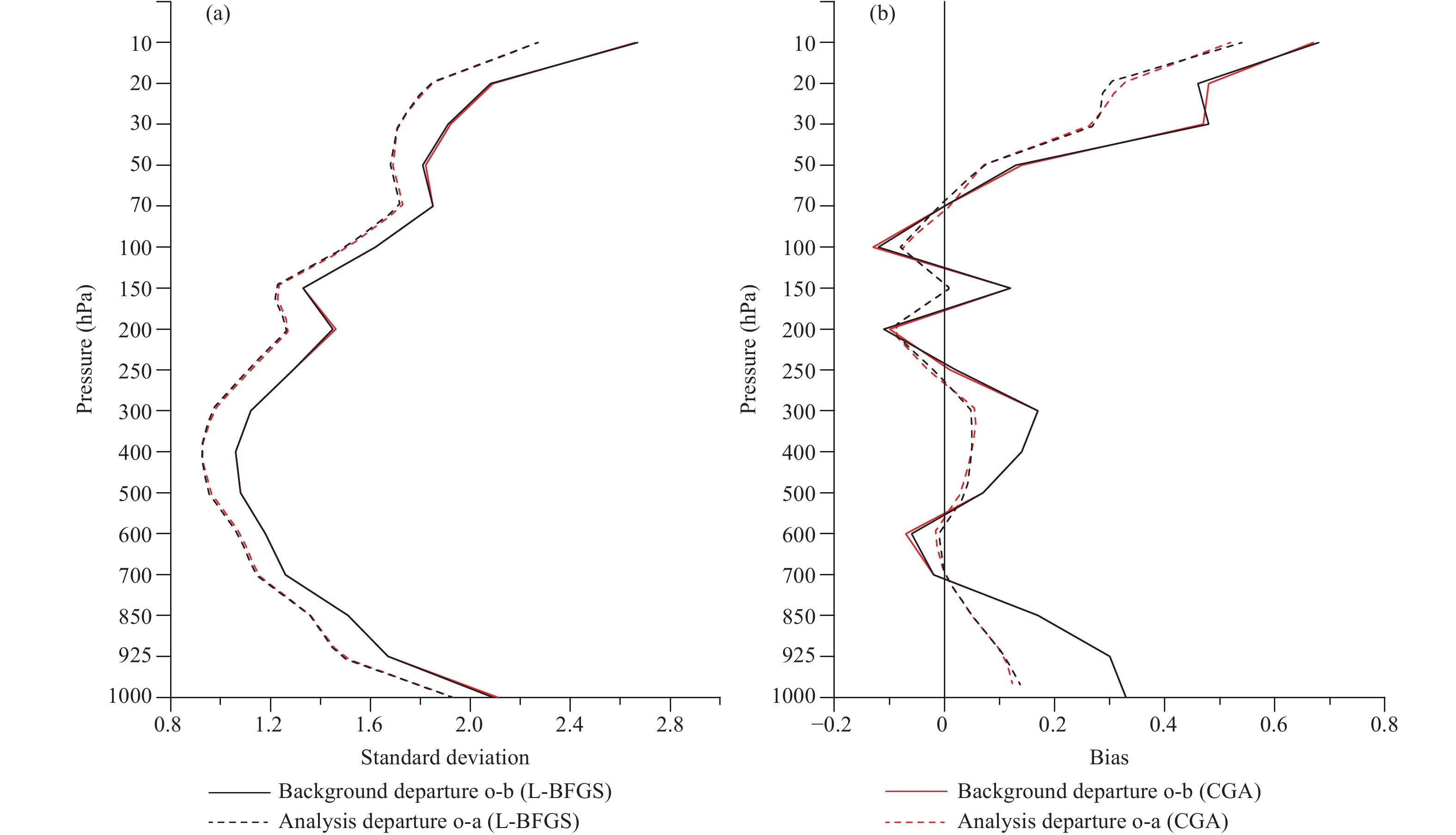
To compare the assimilation results of the batch experiments more reasonably, we exploit the 21-day (from 10 to 30 June 2016) results of the cycling assimilation tests to avoid the influence of the initial field. A statistical analysis of the batch background and analysis deviations from the radiosonde temperature observations for the L-BFGS experiment (shown in black) and the CGA experiment (shown in red) is shown in Fig. 7. The two experiments show very similar standard deviations (Fig. 7a) and biases (Fig. 7b) of the background fields and analysis fields at all levels. In addition, the statistics of the other types of observations between the two experiments are also similar. Therefore, this shows that the estimated solutions [Eq. (1)] for these two minimization algorithms are both reasonable when they reach the same convergence rate in the 4DVar minimization (Fig. 6). This result validates the potential of using these two iterative methods in the GRAPES 4DVar minimization.
|
| Figure 7 (a) Standard deviations and (b) biases of background and analysis fields from radiosonde temperature observations for the L-BFGS experiment (black) and CGA experiment (red) (solid line: background departure o-b; dotted line: analysis departure o-a). |
A CGA based on the Lanczos iteration is investigated in this paper that considers latitudinal and longitudinal grid characteristics under a non-hydrostatic framework in the GRAPES tangent linear and adjoint models. This approach solves the convergence problem through orthogonalization in the Lanczos iteration. The CGA produces equivalent analysis results with far fewer iterations and a higher computational efficiency than the L-BFGS in the batch experiments on the 4DVar system. This conclusion for the GRAPES 4DVar system is consistent with that for the ECMWF 4DVar system. However, the denser grid distribution of GRAPES adds a gradient sensitivity computed by the adjoint model, leading to an increase in the condition number of the Hessian matrix, thereby affecting the convergence rate. However, this issue can be addressed by orthogonalization. Thus, the CGA is more suitable for the operational development of the GRAPES 4DVar system, indicating that the CGA is more suitable for minimization problems such as those in the 4DVar system.
To further improve the convergence of the 4DVar minimization problem, we need to explore the preconditioned CGA based on the eigenvector of the low-resolution minimization, perform additional outer loop updates in the framework of incremental analysis, and ultimately improve the 4DVar analysis technique.
Appendix A: A description of the L-BFGSThe L-BFGS algorithm is an optimization algorithm in the family of quasi-Newton methods that employs a limited amount of computer memory. The algorithm starts with an initial estimate
Step 1. Compute the search direction
Step 2. Set
Step 3. Generate a new search direction
The L-BFGS algorithm attempts to combine modest storage and computational requirements for minimizing
The CGA searches in the direction of conjugated base vectors over the Krylov subspace
The Lanczos approach is applied on the Hessian matrix to iterate and generate a tridiagonal matrix T and an orthogonal matrix Q satisfying the relation
Equating the columns in
| ${J''}{{q}_{k}} = {{\beta }_{{k} - 1}}{{q}_{{k - }{1}}} + {{\alpha }_{k}}{{q}_{k}} + {{\beta }_{k}}{{q}_{{k + }{1}}}.$ | (B1) |
The CGA based on Lanczos iterations starts with an initial estimate
Step 1. Calculate the multiplication of the matrix and vector at the kth step:
| ${{g}_{k}} = {J''}{{q}_{k}},$ | (B2) |
where the largest calculation lies over the whole iterative algorithm because the Hessian matrix is computed using the tangent linear model L and the adjoint model LT, the calculations of which are very large and time consuming.
Step 2. Estimate the kth diagonal element of the matrix T:
| ${{\alpha }_{k}} = \left\langle {{{g}_{k}}, {{q}_{k}}} \right\rangle .$ | (B3) |
Here, the notation
Step 3. Calculate the residual vector:
| ${{r}_{k}} = {{g}_{k}} - {{\alpha }_{k}}{{q}_{k}} - {{\beta }_{{k} - 1}}{{q}_{{k - }{1}}}.$ | (B4) |
Step 4. Calculate the (k+1)th secondary diagonal element of the matrix T:
| ${{\beta }_{k}} = {\left\| {{{r}_{k}}} \right\|_2}, $ | (B5) |
Step 5. Determine the Lanczos vector
| ${{q}_{{k + }{1}}} = {{{{r}_{k}}}/{{{\beta }_{k}}}},$ | (B6) |
which is equivalent to the normalization of the residual vector
Equation (B1) may be written in matrix form as follows:
| ${J''}{{{Q}}_{k}} = {{{Q}}_{k}}{{{T}}_{k}} + {{r}_{k}}{\left({{\mu _k}} \right)^{\rm{T}}},$ | (B7) |
where
| $\delta {{x}_{k}} = \delta {{x}_0} + \sum\nolimits_{{i} = 1}^{k} {\left\langle {{{q}_{i}}, \delta {{y}_{k}}} \right\rangle }.$ | (B8) |
In addition, the eigenvalues and eigenvectors of the Lanczos matrix
Acknowledgments. The authors thank the editor and two anonymous reviewers for their valuable comments and suggestions in improving this manuscript.
| Bannister, R. N., 2017: A review of operational methods of variational and ensemble-variational data assimilation. Quart. J. Roy. Meteor. Soc., 143, 607–633. DOI:10.1002/qj.2982 |
| Clayton, A. M., A. C. Lorenc, and D. M. Barker, 2013: Operationalimplementation of a hybrid ensemble/4D-Var global data assimilation system at the Met Office. Quart. J. Roy. Meteor. Soc., 139, 1445–1461. DOI:10.1002/qj.2054 |
| Courtier, P., J. N. Thépaut, and A. Hollingsworth, 1994: A strategy for operational implementation of 4D-Var, using an incremental approach. Quart. J. Roy. Meteor. Soc., 120, 1367–1387. DOI:10.1002/qj.49712051912 |
| Courtier, P., E. Andersson, W. Heckley, et al., 1998: The ECMWF implementation of three-dimensional variational assimilation (3D-Var). I: Formulation. Quart. J. Roy. Meteor. Soc., 124, 1783–1807. DOI:10.1002/qj.49712455002 |
| Fisher, M., 1998: Minimization algorithms for variational data assimilation. Annual Seminar on Recent Developments in Numerical Methods for Atmospheric Modelling, Shinfield Park, Reading, 7–11 September 1998, ECMWF, 364–385. |
| Fletcher, R., and C. M. Reeves, 1964: Function minimization by conjugate gradients. The Computer Journal, 7, 149–154. DOI:10.1093/comjnl/7.2.149 |
| Golub, G. H., and C. F. Van Loan, 1996: Matrix computations. Mathematical Gazette, 47, 392–396. |
| Gürol, S., A. T. Weaver, A. M. Moore, et al., 2014: B-preconditioned minimization algorithms for variational data assimilation with the dual formulation . Quart. J. Roy. Meteor. Soc., 140, 539–556. DOI:10.1002/qj.2150 |
| Han, J., and H. L. Pan, 2006: Sensitivity of hurricane intensity forecast to convective momentum transport parameterization. Mon. Wea. Rev., 134, 664–674. DOI:10.1175/MWR3090.1 |
| Isaksen, L., M. Bonavita, R. Buizza, et al., 2010: Ensemble of Data Assimilations at ECMWF. ECMWF Technical Memoranda No. 636, Shinfield Park, Reading, 1–48. |
| Janisková, M., J. N. Thépaut, and J. F. Geleyn, 1999: Simplified and regular physical parameterizations for incremental four-dimensional variational assimilation. Mon. Wea. Rev., 127, 26–45. DOI:10.1175/1520-0493(1999)127<0026:SARPPF>2.0.CO;2 |
| Laroche, S., P. Gauthier, M. Tanguay, et al., 2007: Impact of the different components of 4DVAR on the global forecast system of the meteorological service of Canada. Mon. Wea. Rev., 135, 2355–2364. DOI:10.1175/MWR3408.1 |
| Liu, C. S., and Q. N. Xiao, 2013: An ensemble-based four-dimensional variational data assimilation scheme. Part III: Antarctic applications with advanced research WRF using real data. Mon. Wea. Rev., 141, 2721–2739. DOI:10.1175/MWR-D-12-00130.1 |
| Liu, D. C., and J. Nocedal, 1989: On the limited memory BFGS method for large scale optimization. Mathematical Programming, 45, 503–528. DOI:10.1007/BF01589116 |
| Liu, Y. Z., L. Zhang, and Z. Y. Jin, 2017: The optimization of GRAPES global tangent linear model and adjoint model. J. Appl. Meteor. Sci., 28, 62–71. DOI:10.11898/1001-7313.20170106 |
| Lorenc, A. C., S. P. Ballard, R. S. Bell, et al., 2000: The Met. Office global three-dimensional variational data assimilation scheme. Quart. J. Roy. Meteor. Soc., 126, 2991–3012. DOI:10.1002/qj.49712657002 |
| Lorenc, A. C., N. E. Bowler, A. M. Clayton, et al., 2015: Comparison of Hybrid-4DEnVar and Hybrid-4DVar data assimilation methods for global NWP. Mon. Wea. Rev., 143, 212–229. DOI:10.1175/MWR-D-14-00195.1 |
| Nash, S. G., 1984: Newton-type minimization via the Lanczos method. SIAM J. Numer. Anal., 21, 770–788. DOI:10.1137/0721052 |
| Navon, I. M., and D. M. Legler, 1987: Conjugate-gradient methods for large-scale minimization in meteorology. Mon. Wea. Rev., 115, 1479–1502. DOI:10.1175/1520-0493(1987)115<1479:CGMFLS>2.0.CO;2 |
| Paige, C. C., 1970: Practical use of the symmetric Lanczos process with re-orthogonalization. BIT Numerical Mathematics, 10, 183–195. DOI:10.1007/BF01936866 |
| Paige, C. C., and M. A. Saunders, 1982: LSQR: An algorithm for sparse linear equations and sparse least squares. ACM Transactions on Mathematical Software, 8, 43–71. DOI:10.1145/355984.355989 |
| Parlett, B. N., and D. S. Scott, 1979: The Lanczos algorithm with selective orthogonalization. Mathematics of Computation, 33, 217–238. DOI:10.1090/S0025-5718-1979-0514820-3 |
| Rabier, F., 2005: Overview of global data assimilation developments in numerical weather-prediction centres. Quart. J. Roy. Meteor. Soc., 131, 3215–3233. DOI:10.1256/qj.05.129 |
| Rabier, F., A. McNally, E. Andersson, et al., 1998: The ECMWF implementation of three-dimensional variational assimilation (3D-Var). II: Structure functions. Quart. J. Roy. Meteor. Soc., 124, 1809–1829. DOI:10.1002/qj.49712455003 |
| Rabier, F., H. Järvinen, E. Klinker, et al., 2000: The ECMWF operational implementation of four-dimensional variational assimilation. I: Experimental results with simplified physics. Quart. J. Roy. Meteor. Soc., 126, 1143–1170. DOI:10.1002/qj.49712656415 |
| Rawlins, F., S. P. Ballard, K. Bovis, et al., 2007: The Met Office global four-dimensional variational data assimilation scheme. Quart. J. Roy. Meteor. Soc., 133, 347–362. DOI:10.1002/qj.32 |
| Shen, X. S., Y. Su, J. L. Hu, et al., 2017: Development and operation transformation of GRAPES global middle range forecast system. J. Appl. Meteor. Sci., 28, 1–10. DOI:10.11898/1001-7313.20170101 |
| Simon, H. D., 1984: The Lanczos algorithm with partial reorthogonalization. Mathematics of Computation, 42, 115–142. DOI:10.1090/S0025-5718-1984-0725988-X |
| Talagrand, O., and P. Courtier, 1987: Variational assimilation of meteorological observations with the adjoint vorticity equation. I: Theory. Quart. J. Roy. Meteor. Soc., 113, 1311–1328. DOI:10.1002/qj.49711347812 |
| Thépaut, J. N., R. N. Hoffman, and P. Courtier, 1993: Interactions of dynamics and observations in a four-dimensional variationalassimilation. Mon. Wea. Rev., 121, 3393–3414. DOI:10.1175/1520-0493(1993)121<3393:IODAOI>2.0.CO;2 |
| Tompkins, A. M., and M. Janisková, 2004: A cloud scheme for data assimilation: Description and initial tests. Quart. J. Roy. Meteor., 130, 2495–2517. DOI:10.1256/qj.03.162 |
| Trémolet, Y., 2007: Incremental 4D-Var convergence study. Tellus A: Dynamic Meteorology and Oceanography, 59, 706–718. DOI:10.1111/j.1600-0870.2007.00271.x |
| Xue, J. S., S. Y. Zhuang, G. F. Zhu, et al., 2008: Scientific design and preliminary results of three-dimensional variational data assimilation system of GRAPES. Chinese Science Bulletin, 53, 3446–3457. DOI:10.1007/s11434-008-0416-0 |
| Zhang, L., and Y. Z. Liu, 2017: The preconditioning of minimization algorithm in GRAPES global four-dimensional variational data assimilation system. J. Appl. Meteor. Sci., 28, 168–176. DOI:10.11898/1001-7313.20170204 |
| Zou, X., I. M. Navon, M. Berger, et al., 1993: Numerical experience with limited-memory Quasi-Newton and Truncated New-ton methods. SIAM J. Optim., 3, 582–608. DOI:10.1137/0803029 |
 2018, Vol. 32


