The Chinese Meteorological Society
Article Information
- WEI, Ting, Jian LI, Xinyao RONG, et al., 2018.
- Arctic Climate Changes Based on Historical Simulations (1900‒2013) with the CAMS-CSM. 2018.
- J. Meteor. Res., 32(6): 881-895
- http://dx.doi.org/10.1007/s13351-018-7188-5
Article History
- Received January 10, 2018
- in final form July 30, 2018
2. School of Atmospheric Sciences, Sun Yat-Sen University, Guangzhou 510275;
3. Zhuhai Joint Innovative Center for Climate–Environment–Ecosystem, Future Earth Research Institute, Beijing Normal University, Zhuhai 519087;
4. Center for Excellence in Tibetan Plateau Earth Sciences, Chinese Academy of Sciences, Beijing 100101;
5. Institute of Atmospheric Sciences, Fudan University, Shanghai 200000
The Arctic climate system contains close interactions among the atmosphere, ocean, and cryosphere, and has experienced unprecedented changes within the past few decades. Reductions in Arctic snow and ice contribute to the Arctic amplification, which is characterized by a warming rate in the Arctic being more than twice that in the tropics and midlatitudes (Manabe and Wetherald, 1975; Screen, 2014). Arctic warming results in dramatic melting of glaciers and ice sheets (e.g., Yan et al., 2014), which leads to the export of freshwater from the Arctic to North Atlantic altering the variability of the ocean meridional overturning circulation (Dickson et al., 1988; Holland et al., 2001). The thawing of Arctic permafrost increases the release of methane and soil organic carbon, which aggravates global warming in turn (Schuur et al., 2015; Guo and Wang, 2017). In addition, profound Arctic changes have influenced the midlatitude climate conditions via dynamic pathways (Deser et al., 2010; Wu et al., 2015), which contributes to more frequent extreme weather events (Cohen et al., 2014; Wei et al., 2016).
Climate modelling is one of the most important means to study climate change in the Arctic and its impacts. First, it is important to assess the capability of the climate model to simulate the Arctic climate system. The state-of-the-art models in the Coupled Model Intercomparison Project Phase 5 (CMIP5) generally perform well in depicting the majority of observed climatic features, but some biases still exist in the Arctic (Vaughan et al., 2013). Although climate models are able to reproduce the increasing trend in the global mean temperature during the historical period (1870–2005), most of them tend to underestimate the warming trend in the Arctic. In addition, CMIP5 models show low skill in depicting precipitation, especially at the regional scale (Rougier et al., 2009; Neelin et al., 2010). The multi-model ensemble mean of the CMIP5 models captures the seasonal cycles of the Arctic sea–ice extent (SIE) and snow cover extent (SCE) but overestimates the total SIE (~10%) and underestimates the SCE in the Northern Hemisphere (Vaughan et al., 2013). The biases of snow and ice and their associated temperature feedbacks are closely linked with the simulated biases for Arctic amplification (Pithan and Mauritsen, 2014).
The Chinese Academy of Meteorological Sciences Climate System Model (CAMS-CSM; Rong et al., 2018) is a newly developed global climate model that will participate in the CMIP6. Recently, many studies have been devoted to evaluate the model capability in reproducing the present-day climate, but the model performance in the Arctic remains unknown. Given the importance of Arctic climate modelling, in this study, we evaluate the skills of the CAMS-CSM in modelling the Arctic climate system based on historical simulations (1900–2013). These results could reveal the capability of the CAMS-CSM over the Arctic and provide effective information for model improvement. Section 2 provides descriptions of the model and observation datasets. Section 3 documents the performance of the CAMS-CSM in simulating the Arctic atmosphere, ocean, and cryosphere throughout a historical period. The main results are summarized in Section 4.
2 Data and methods 2.1 Observational datasetsThe seven observation-based datasets are employed in this study, including (1) 2-m air temperature from the latest global atmospheric reanalysis produced by the ECMWF reanalysis (ERA-Interim; Dee et al., 2011), where the ERA-Interim dataset (~1° × 1°) uses an improved atmospheric model and assimilation system based on those used in ERA-40 and extends back to 1979; (2) 1000-hPa geopotential heights from the NOAA/NCEP–DOE reanalysis II, where the NCEP2 dataset (2.5° × 2.5°) is an improved version of the NCEP–NCAR reanalysis I dataset and covers the period from 1979 to present (https://www.esrl.noaa.gov/psd/); (3) Global Precipitation Climatology Project (GPCP) monthly rainfall at a 2.5° × 2.5° resolution from 1979 to the present (Adler et al., 2003), where the GPCP dataset merges precipitation data from rain-gauge stations, satellites, and sounding observations and is one of the most-used precipitation datasets for climate studies; (4) global decadal averages of the climatological mean ocean temperature (Locarnini et al., 2013) and salinity (Zweng et al., 2013) from the World Ocean Atlas 2013 (WOA13), where the WOA13 has 102 standard depth levels from 0–5500 m with a 1° horizontal resolution, is based on in situ measurements from a wide variety of sources and generally represents large-scale features of the global ocean quite well; (5) global ocean heat content (OHC) at depths of 0–700 m from 1955 to present (Levitus et al., 2012), where the calculated OHC derives from updated data from the World Ocean Database (Boyer et al, 2009) and improved ARGO profiling data; (6) the snow cover extent climate data record by Rutgers, with a nominal resolution of ~190.5 km at a standard parallel of 60°N (Robinson et al., 2012), where the data are combined with historical digitized analyses based on visual inspection and modern multi-spectral remote sensing that spans from 1967 to present; and (7) the UK Meteorological Office Hadley Centre sea ice dataset version 1 (HadISST1), which has a 1° × 1° resolution (Rayner et al., 2003) and combines data using historical ice charts on shipping, expeditions, other activities, passive microwave satellite retrievals, and NCEP operational ice analyses.
2.2 CAMS-CSM model and its historical experimentThe CAMS-CSM is a fully coupled global climate model that provides state-of-the-art computer simulations of the earth’s climate. The atmospheric component of the CAMS-CSM is a modified version of ECHAM5, which is a general circulation model developed by the Max Planck Institute for Meteorology (Roeckner et al., 2003; Cao et al., 2015). The modified ECHAM5 uses a two-step shape-preserving advection scheme (Yu, 1994) and the k-distribution radiation transfer parameterization (Zhang and Li, 2016), which contribute to the reduced biases in precipitation over the steep edges of the Tibetan Plateau. The resolution of the modified ECHAM5 is T106L31, which is equal to a horizontal resolution of ~1° × 1° and has 31 vertical layers extending from the surface to 10 hPa. The land component comprises the modified Common Land Model (CoLM; Dai et al., 2003). The unfrozen water process (Niu and Yang, 2006) is adopted in the modified version of this model to allow liquid water and ice to coexist in the soil below the freezing point, which has been proven to have profound impacts on the East Asian climate (Xin et al., 2012). The modified CoLM shares the same horizontal grid as the modified ECHAM5 and has 10 uneven vertical soil layers from the surface to a 3-m depth. The ocean model and sea–ice model derive from the Geophysical Fluid Dynamic Laboratory Modular Ocean Model version 4 (MOM4; Griffies et al., 2004) and sea ice simulator (SIS; Winton, 2000), respectively. The zonal resolution of MOM4 is 1° globally, and the meridional resolution is ~1° (1/3° at the equator). There are 23 even layers in the upper ocean (0–230 m) within 50 vertical layers. The SIS is a dynamic sea–ice model with a three-layer structure similar to the Semtner scheme (Winton, 2000). The heat capacity is zero in the snow layer, variable in the upper ice layer (for describing brine pockets), and fixed in the lower ice layer. Snow and ice layer thicknesses and upper and lower ice layer temperatures are prognostic variables. The brine pockets are determined by the upper ice temperature and predefined ice salinity. The surface temperature is defined by the balance between the upward and conductive heat fluxes. The sea ice in each grid is comprised by five categories and could be redistributed by an enthalpy conserving approach. The internal stresses of ice are calculated by the elastic–viscous–plastic technique (Hunke and Dukowicz, 1997). The SIS shares the same horizontal grid set as that of MOM4. The Flexible Modelling System (FMS) coupler is used for flux calculations and interpolations between each component of the CAMS-CSM.
The historical simulation via the CAMS-CSM is conducted with standard forcing datasets of the CMIP6 (Eyring et al., 2016). The simulation spans from 1900 to 2013. Monthly and daily outputs are achieved for further analysis. Note that initial conditions (ICs) from the pre-industrial control experiment are used to start the historical experiment from 1900. It is not precise because of the climate drift. However, given the relative small radiative forcings from 1850 to 1900 compared with that from 1900–2013, the Arctic simulation during the evaluation period (1979–2013) cannot be largely affected by the biases from ICs.
3 Results 3.1 Arctic atmosphere 3.1.1 Surface air temperatureThe observed climatological surface air temperature (T2m) in the Arctic shows a significant zonal distribution that decreases with increasing latitude. In addition, there is a low temperature center over Greenland that is covered by an extensive ice sheet (Fig. 1a). The modelled annual mean temperature during 1979–2013 resembles those from the observations (Fig. 1b), with a pattern correlation coefficient of 0.94 and a root-mean-square error (RMSE) of 0.85°C. However, the simulated temperatures from Greenland to the Barents Sea and those over the Rocky Mountains exhibit obvious cold biases (Fig. 1c).

|
| Figure 1 Annual mean surface air temperature (T2m; °C) over the period 1979‒2013 based on the (a) ERA-Interim dataset and (b) simulation via the CAMS-CSM. (c) Differences in surface air temperature (°C) between the simulations and observations. |
The observed T2m shows a decreasing trend in the Bering Sea and an overall increasing trend with maximum centers located over the Barents Sea, northeastern Canada and Baffin Bay (Fig. 2a). Compared with the observations, CAMS-CSM displays a similar warming trend within the Arctic Circle and a much larger one south of ~60°N (Figs. 2a–c). This result implies a weakened Arctic amplification via the CAMS-CSM. This phenomenon is more clearly observed from the zonal mean temperature trend (Fig. 2d). The simulation and observation have similar warming trends that increase with increasing latitude. However, the model overestimates the warming trend south of ~60°N [0.34°C (10 yr)–1 vs. 0.03°C (10 yr)–1], while it captures the trend in the Arctic compared to the observations. Because many researchers have proposed that surface albedo feedback is the main contributor to Arctic amplification (Screen and Simmonds, 2010; Crook et al., 2011), the simulations of snow and sea ice and their linkages and biases for Arctic amplification are discussed in the following sections. Figure 2e compares the simulated temporal evolution of T2m in the Arctic with the observations. There is a significant warming trend during the past 35 years [0.38°C (10 yr)–1]. Although the model captures the long-term warming trend [0.39°C (10 yr)–1], there are remarkable biases in interannual variability. In summary, the CAMS-CSM reproduces the climatological features of the Arctic annual mean surface temperature throughout the historical period and rapid warming during the past 35 years. A disagreement largely exists in local areas and the magnitude of the Arctic amplification.

|
| Figure 2 Linear trends in surface air temperature over the period 1979‒2013 [°C (10 yr)–1] based on the (a) observations (ERA-Interim) and (b) simulation via the CAMS-CSM. (c) Differences in the linear trends [°C (10 yr)–1] between the simulations and observations. (d) Zonal mean air temperature trends over the period 1979–2013. (e) The evolution of Arctic surface air temperature anomalies (°C; relative to 1979–2013) for the period 1901–2013; the thin lines represent the annual mean, and the thick lines represent the five-point running means. |
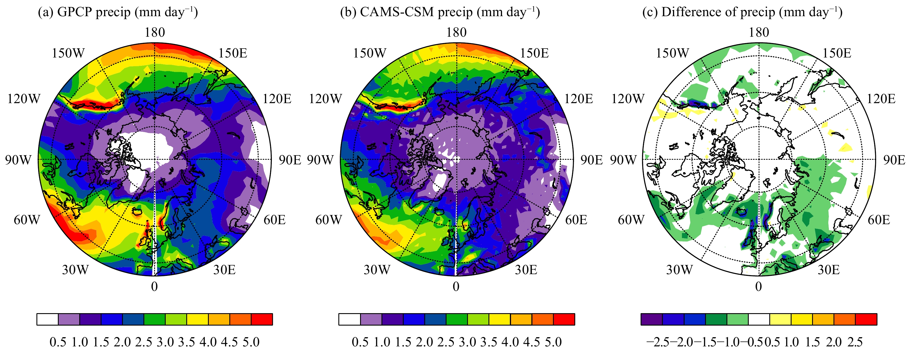
The simulation of precipitation is challenging for climate models, as it depends heavily on processes that must be parameterized (Hartmann et al., 2013). Spatial heterogeneity caused by surface conditions (e.g., topography and vegetation) cause precipitation modelling at a regional scale to become more difficult. Precipitation in the Arctic tends to be smaller towards higher latitudes. The most intense precipitation in the Arctic is located in the regions of southeastern Greenland, Scandinavia, and the Coast Mountains, with a minimum precipitation center over the Arctic Ocean (Fig. 3a). Figures 3b and 3c show the annual mean precipitation simulated by the CAMS-CSM and the biases relative to the GPCP. The large-scale pattern is well captured by the model (e.g., decreasing precipitation with increasing latitude). The refined resolution of the CAMS-CSM helps the model reproduce the major regional features of precipitation (e.g., the precipitation centers over southeastern Greenland, Scandinavia, and the Coast Mountains) (Fig. 3b). The pattern correlation coefficient between the simulations and observations is 0.86, with an RMSE of 0.63 mm day–1. Because the regional precipitation simulation has strong parameter and resolution dependence (Rougier et al., 2009; Yan et al., 2016), some precipitation biases still persist over the coastal regions and surrounding oceans (Fig. 3c).
|
| Figure 3 As in Fig. 1, but for annual mean precipitation (precip; mm day–1). |
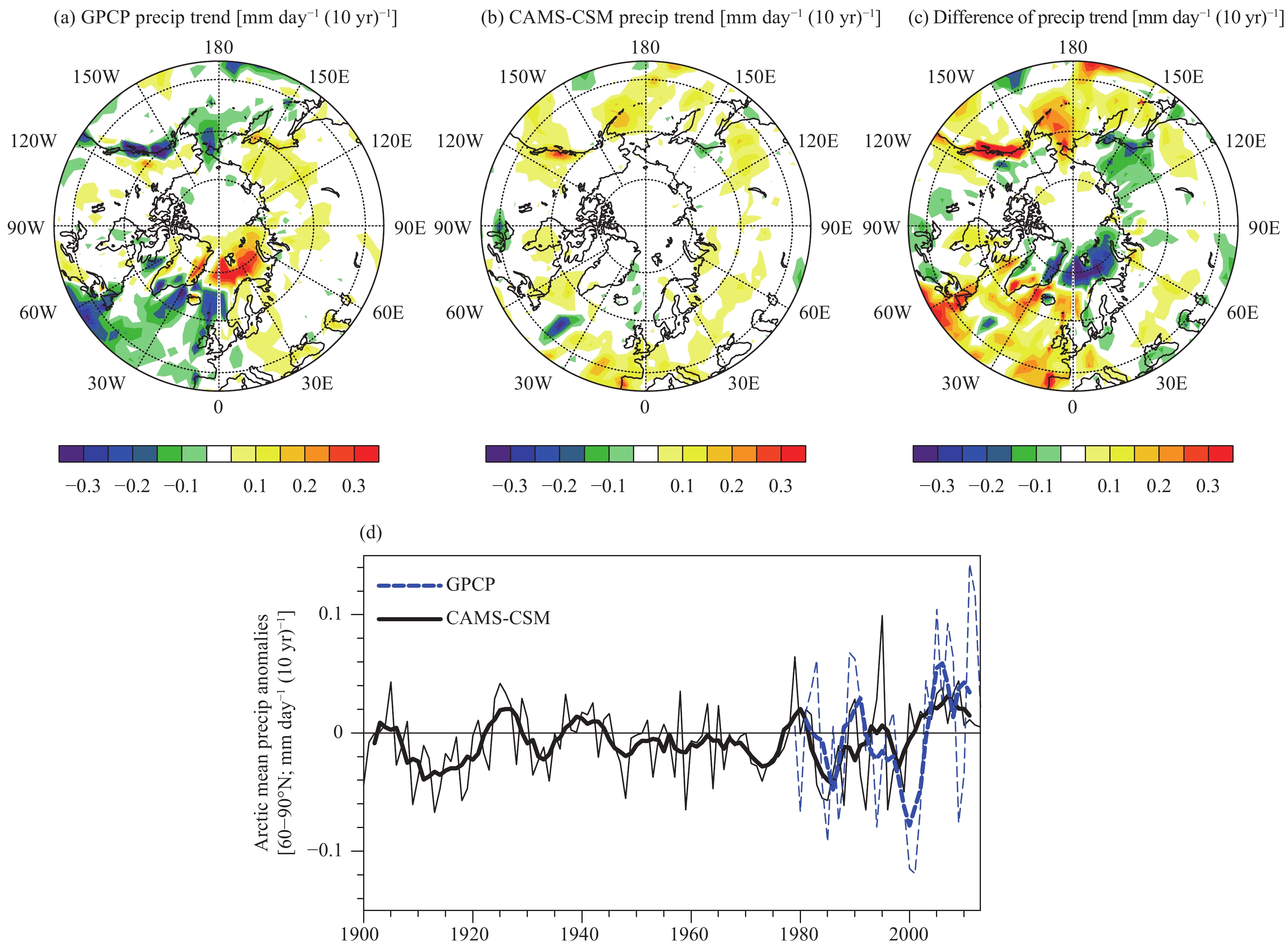
Figure 4 shows the spatial pattern of the annual mean precipitation trend during 1979–2013. The observed precipitation trend in the Arctic shows a regionally discrete pattern, with an increasing trend in most regions that is coupled with a decreasing trend along western coastlines (Fig. 4a). Limited by resolution and the land–sea distribution of the model, the CAMS-CSM fails to capture the magnitude of the precipitation change in most regions, including the decreasing trend over the Coast Mountains, Greenland Sea, and Norwegian Sea and the increasing trend over the Barents Sea (Figs. 4b, c). As shown in Fig. 4d, precipitation averaged over the Arctic shows an overall positive trend [5.84 mm (10 yr)–1] with interdecadal fluctuations since 1979. This evolution pattern is roughly reproduced by the CAMS-CSM, but the model tends to underestimate the increasing trend [3.65 mm (10 yr)–1], especially since the 2000s.
|
| Figure 4 Linear trends in precipitation [precip; mm day–1 (10 yr)–1] over 1979–2013 based on the (a) observations (GPCP) and (b) simulation via the CAMS-CSM. (c) Differences in linear trends [mm day–1 (10 yr)–1] between the simulations and observations. (d) The evolution of the Arctic mean precipitation anomalies (mm day–1; relative to 1979–2013) for the period 1900–2013; the thin lines represent the annual mean, and the thick lines represent the five-point running means. |
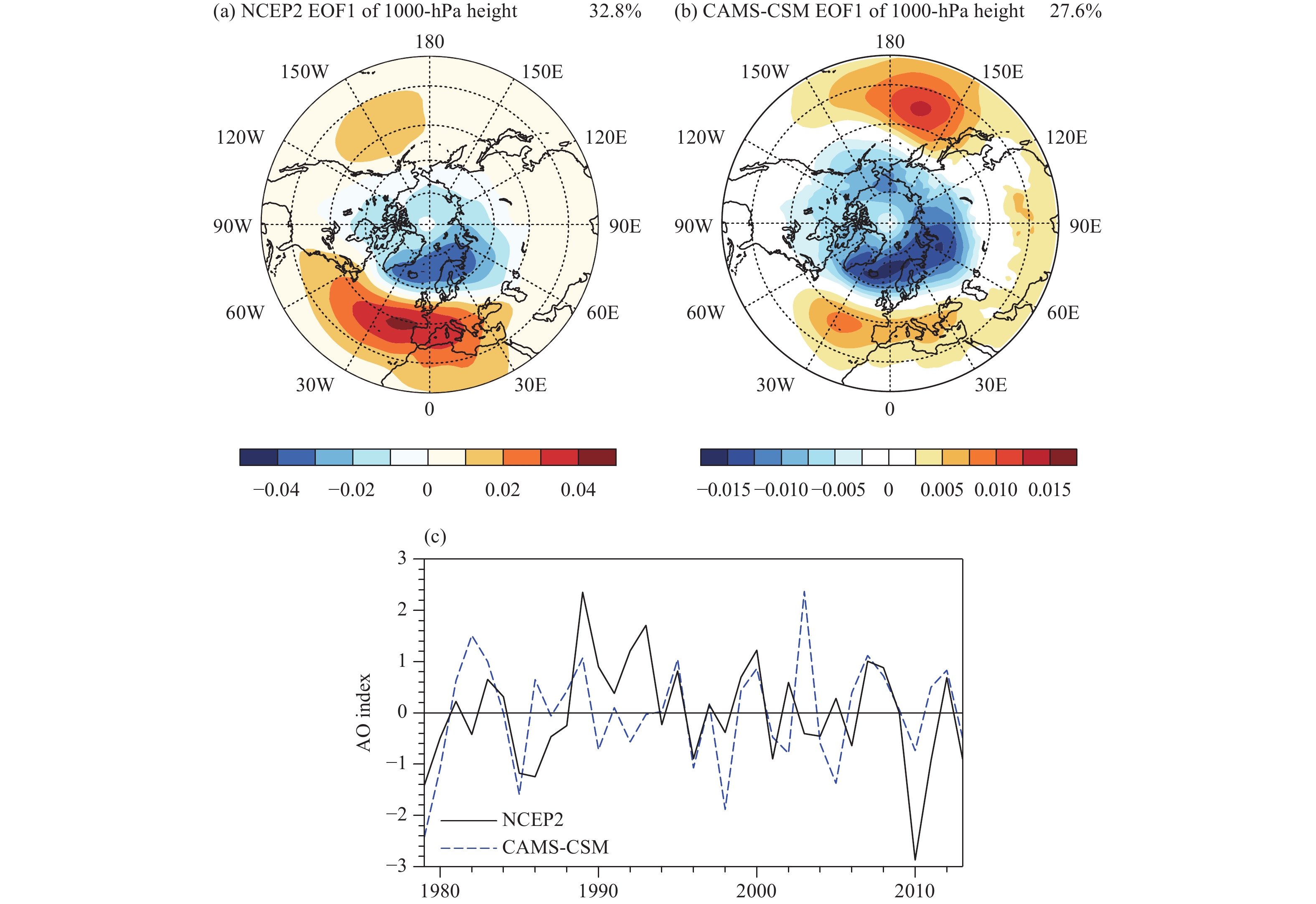
The AO represents the primary pattern during winter at a 1000-hPa height and has a zonally symmetric structure (Thompson and Wallace, 1998). Previous studies have revealed that the winter AO has a close relation to surface air temperature over the Arctic and Eurasian continents (Thompson and Wallace, 1998; Wang and Ikeda, 2000). The CAMS-CSM reproduces the AO pattern with a negative height anomaly over the Arctic and a positive anomaly over midlatitudes (Fig 5). However, the model underestimates the percent variance associated with the leading eigenvalue (27.6%) compared with the observed one (32.8%). The correlation coefficient between the simulated and observed AO index is 0.38 at the 5% significance level. As a result, Arctic atmospheric circulation can be reproduced by the CAMS-CSM with reasonable patterns and variability.
|
| Figure 5 The primary pattern of 1000-hPa height anomalies poleward of 20°N in winter based on the (a) observations (NCEP2) and (b) simulation via the CAMS-CSM with the percent variance associated with the leading eigenvalue. (c) The evolution of the standardized AO index for the period 1979–2013. |
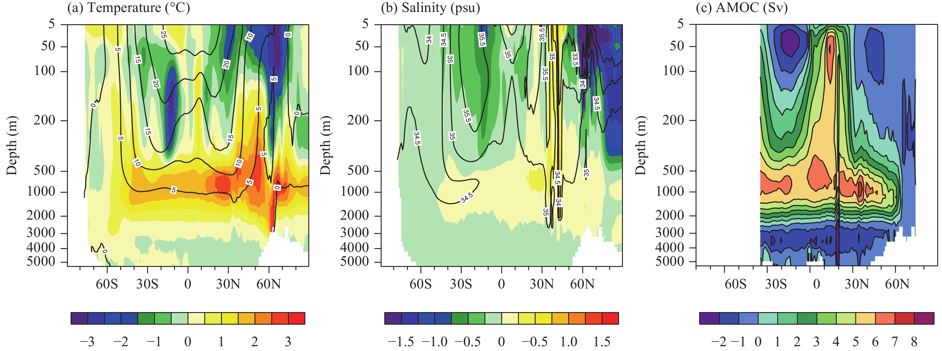
The Arctic region is composed of the Arctic Ocean, sea–ice cover, and surrounding continents. The accurate simulation of the Arctic Ocean is essential for modelling the variations in Arctic climate conditions and sea ice. Given that the Arctic Ocean is largely covered with sea ice, we evaluate the vertical distribution of the ocean potential temperature rather than the SST. Figures 6a and 6b show the observed climatological potential temperature and salinity and the differences between the CAMS-CSM and observations during 1975–2012. The observed ocean temperature from WOA13 presents a notable increase from –1.8°C at the surface to 0°C at a 200-m depth and remains constant below 200 m in the Arctic Ocean. The model reproduces the distribution of ocean temperatures in the Arctic, with a pattern correlation coefficient of 0.72 and an RMSE of 0.94°C. However, the zonally averaged ocean temperature is underestimated at depths ranging from 200 to 500 m but is overestimated at depths of 500–2000 m (Fig. 6a). This anomalous pattern is similar to that of the ensemble mean of CMIP5 models (Flato et al., 2013) but with smaller biases, indicating the relatively better skill of the CAMS-CSM for the Arctic Ocean.
Salinity at the sea surface resembles an evaporation–precipitation pattern, with some differences due to runoff, ocean currents and ice melt (Talley, 2002). The range of salinity for the open ocean surface is approximately 30–40 psu according to the WOA13 dataset. The lowest salinities occur in the Arctic and Antarctic, where there is both net precipitation and seasonal ice melt. Salinities from the sea surface are carried by water flow down into the interior of the ocean, indicating the sources and pathways of the circulation. The data-model comparisons show that CAMS-CSM largely underestimates salinity in the upper level of the Arctic Ocean (Fig. 6b), with an RMSE of 1.97 psu. Given the relatively smaller bias in Arctic precipitation (Fig. 3c), the large bias of salinity in the Arctic Ocean might be attributed to the simulation deviation for sea ice (Fig. 10c). Increased seasonal ice melt could reduce the salinity in the Arctic Ocean.
The Atlantic meridional overturning circulation (AMOC) plays a central role in the global climate via heat and fresh water transport. In North Atlantic (north of 40°N) and around the Barents Sea, excessive fresh water in the CAMS-CSM reduces local convection and weakens the AMOC. Figure 6c shows that the CAMS-CSM simulates weak tropical–subtropical cells above 500 m and the North Atlantic Deep Water (NADW) mass between 500 and 2500 m and north of 35°S compared with the observed values (Lumpkin and Speer, 2007). The simulated maximum transport magnitude of the NADW is approximately 14 Sv, which is located at approximately 35°N (between 800 and 1000 m). At 26.5°N, the simulated maximum transport magnitude of the NADW is approximately 9.6 Sv, which is less than the observed value (18.5 ± 5.6 Sv; Cunningham et al., 2007). At 41°N, the average transport magnitude is 9.0 Sv, which is less than the observation value (15.5 ± 2.4 Sv; Willis, 2010).
The simulated 0–700-m OHC by the CAMS-CSM is compared with the observations in Fig. 7. The model reproduces a remarkable upward trend in global OHC since 1955 but underestimates the magnitude (Fig. 7a). The observed Arctic OHC presents obvious interdecadal variations with a long-term increasing trend, although this trend is smaller than that of the global mean. There is, however, no significant trend in the Arctic OHC via the simulation (Fig. 7b). The model biases in the Arctic impact the simulation of the Arctic cryosphere (Steele et al., 2010) and temperature-related feedbacks, which potentially affects long-term projections (Steinacher et al., 2009).

|
| Figure 7 As in Fig. 3, but for the 0–700-m OHC in (a) the global and (b) Arctic. |
The cryosphere, which contains a substantial fraction of water in the frozen state, is the most distinctive feature of the Arctic climate system. The cryosphere, which is sensitive to temperature changes, determines the partitioning of surface radiation, the water cycle and sea level (Vaughan et al., 2013). Given the lack of ice-sheet models and refined hydrological models in the CAMS-CSM, we pay attention to the simulations of snow and sea ice in this section.
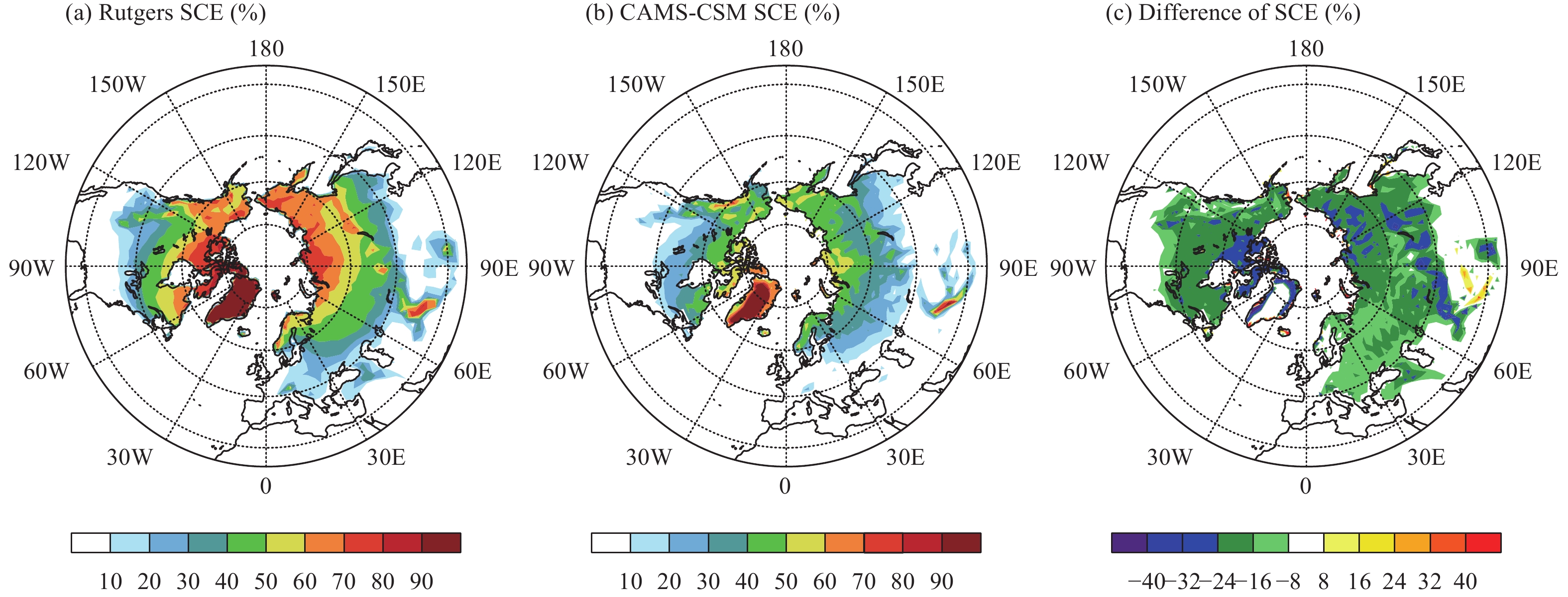
3.3.1 Snow coverFigure 8 shows the annual mean SCE during 1979–2013 for the simulation via the CAMS-CSM, the observations and their differences. The observed SCE in the Northern Hemisphere (NH) illustrates a poleward increase in SCE, with the most snow cover over Greenland and the Himalayas. The CAMS-CSM reproduces the spatial distribution of the climatological SCE, with a pattern correlation coefficient of 0.86, but underestimates the SCE across the NH, with the largest biases located at the marginal areas of Greenland and northeast Canada. An important factor that influences the SCE is the impurities in the snow surface, which have size-dependent thermomechanical effects that are poorly described in the CoLM. This defect in the model could change the radiative balance at the surface, leading to biases in the SCE. In addition, regional biases might also link with unresolved steep topographies in the model and uncertainties in the observations (Vaughan et al., 2013).
|
| Figure 8 As in Fig. 1, but for the annual mean SCE (%). |
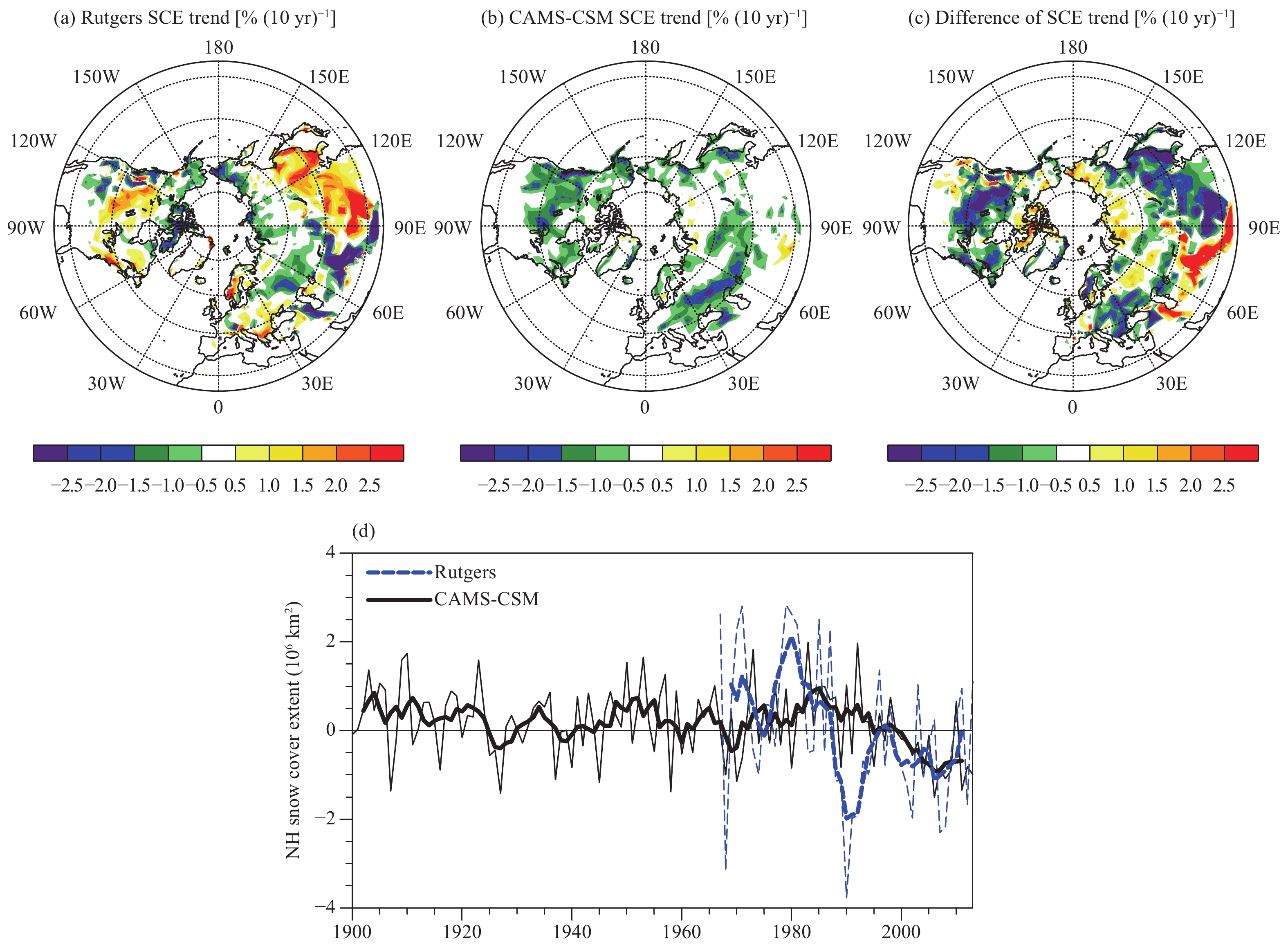
Despite the reasonable pattern of the climatological mean SCE, there are significant biases in the trend of SCE in most regions. The observed SCE shows remarkable positive trends in Mongolia, eastern Tibetan Plateau, and eastern Canada, and negative trends in the Arctic Circle and western Tibetan Plateau (Fig. 9a). The CAMS-CSM simulates an overall negative trend, with the largest magnitude occurring over western Siberia and Canada (Fig. 9b). Additionally, there are larger SCE biases over the mid- to high-latitudes outside of the Arctic Circle, where snow cover is sparse (Fig. 9c). These biases might be partially attributed to the complex interactions between the plant canopy and snow cover (Rutter et al., 2009) in mid- to high-latitude regions.
The spring SCE has larger decreasing trends and higher snow albedo feedbacks than those in other seasons (Najafi et al., 2016). The decrease SCE in spring, which has contributed to both the increase in warm season surface temperatures over Northern Hemisphere extratropical landmasses and the decrease in summer Arctic sea ice (Cohen et al., 2014), is considered to be a climatic indicator. Figure 9d shows the time series of the observed and simulated NH snow cover area in March and April. The observed SCE presents a remarkable decreasing trend since 1979 [–0.52 × 10⁶ km2 (10 yr)–1], with significant interannual and interdecadal variability. The CAMS-CSM reproduces a decreasing trend in the SCE with a similar amplitude [–0.52 × 10⁶ km2 (10 yr)–1]. However, the interdecadal variations in SCE related to the internal variability of the climate system (Bojariu and Gimeno, 2003) are not well depicted by the model.
|
| Figure 9 As in Fig 4, but for the SCE (km2). |
The most reliable, measured feature of sea ice is the SIE. In the Arctic, a large sea surface area is covered by sea ice, except for the Norwegian Sea, where the AMOC results in warmer SSTs. Compared with the observations, the CAMS-CSM broadly captures the large-scale distribution of sea ice, with a pattern correlation coefficient of 0.93 and an RMSE of 0.93% (Fig. 10). However, the model overestimates the SIE in most regions, especially over the Labrador Sea, Greenland Sea and Barents Sea. It closely links to simulated cold biases in these oceans with a weaker AMOC (Fig. 6c). These biases could lead to a colder sea surface and weaker poleward transport, contributing to a larger SIE.
|
| Figure 6 The vertical distributions of zonally averaged ocean (a) potential temperature (°C) and (b) salinity (psu) during 1975–2012 in the observations (contours) and simulation (shading). (c) AMOC in the simulation. |
The SIE is well-measured by satellite, while monitoring sea–ice thickness and snow thickness over sea–ice regions has been and remains a challenge. Therefore, the simulated ice and snow thicknesses are shown in Fig. 10 without the observations. Note that the distribution of ice thickness shows a similar pattern with that of SIE. Snow thickness over the sea–ice region shows a large center from the Greenland Sea to Svalbard. Due to the high albedo of snow, local air becomes colder, and SIE further expands through a large positive feedback, which also contributes to colder Arctic (Fig. 1c) and weaker amplification effects.

|
| Figure 10 (a–c) As in Fig. 1, but for the SIE (%). (d) Annual mean sea ice thickness and (e) snow thickness over sea ice during 1979‒2013 based on the simulation by the CAMS-CSM. |
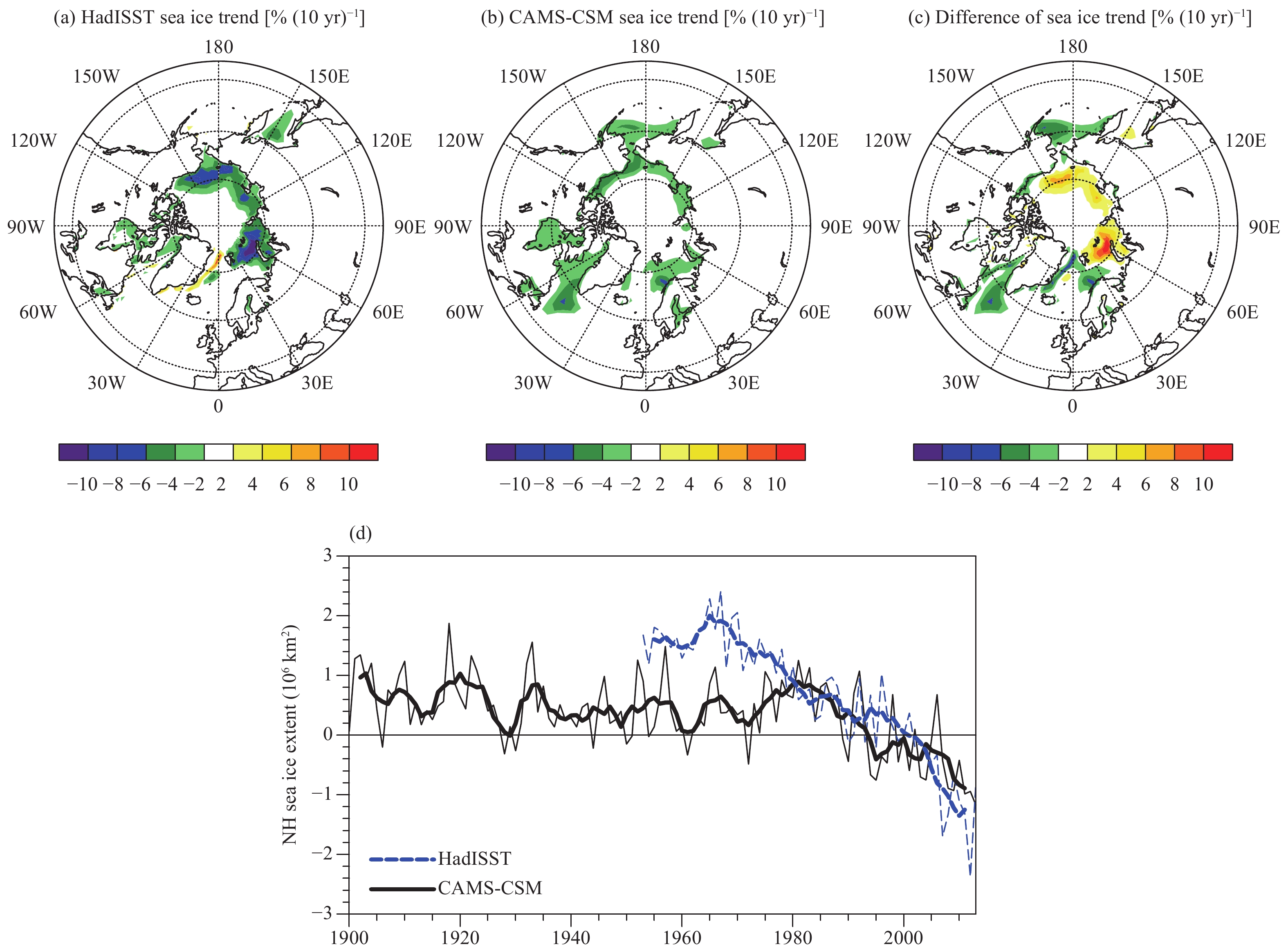
There is a significant decreasing trend in SIE in the NH over the past 30 years, especially over the Barents Sea, Kara Sea, and Chukchi Sea (Fig. 11a). Notable features of the simulation are overestimations of the trends in the aforementioned regions and underestimations in other regions (Figs. 11b, c). In addition, the CAMS-CSM underestimates the overall decreasing trend in Arctic sea ice in September (Fig. 11d) since 1953 [–0.51 × 10⁶ km2 (10 yr)–1 in the observation vs. –0.2 × 10⁶ km2 (10 yr)–1 in the simulation], which is similar to the biases in most of the CMIP5 models (Flato et al., 2013). Because sea ice is a product of air–sea interactions, which are still poorly quantified (Vaughan et al., 2013), the biases of the simulated SIE might be attributed to several factors, such as the description of heat transport by ocean currents (Melsom et al., 2009), high-latitude processes (e.g., polar winds and clouds; Rampal et al., 2009), and several processes not yet included in the models (e.g., deposition of black carbon; Ramanathan and Carmichael, 2008). In addition, underestimated sea–ice trends might contribute to the underestimation of Arctic amplification by the CAMS-CSM in Fig. 2.
|
| Figure 11 As in Fig. 4, but for the SIE (km2). |
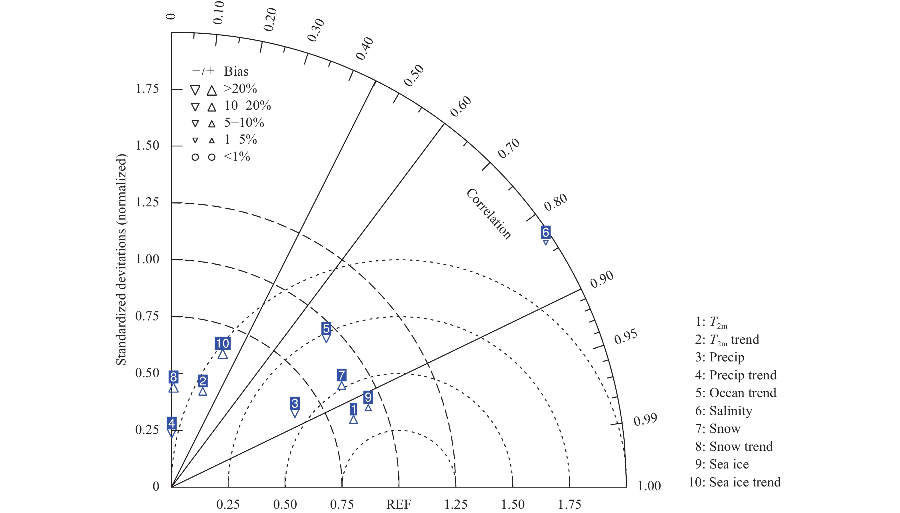
The Taylor diagram (Taylor, 2001) is adopted to evaluate the overall performance of model in simulating the Arctic climate (Fig. 12). In a Taylor diagram, the “REF” point at a unit distance from the origin point on the horizontal axis is denoted as the observed field. The standard deviation of the modelled field is the radial distance from the origin. The centered RMSE, which is used to quantify the pattern biases between the simulations and observations, is equal to the distance to the observed point. The azimuthal position gives the spatial correlation coefficient between the observed and corresponding simulation fields. Note that the centered RMSE and modelled standard deviation have been normalized by the observed standard deviation. In addition, the percent bias is calculated as bias = 100 × (Meanmodel–Meanobs)/Meanobs (http://www.ncl.ucar.edu/).
As shown in Fig. 12, the CAMS-CSM shows a better performance in the simulation of surface air temperature and precipitation from 60° to 90°N, SCE, and SIE in the NH. The pattern correlations between the simulations and observations are greater than 0.85, and the RMSEs are less than 0.75, indicating a good performance of the CAMS-CSM in modelling spatial distributions and its variabilities. However, the model performs poorly in simulating the salinity of the Arctic Ocean, with a large RMSE. In addition, the model shows little skill in capturing the distributions of linear trends, with very low correlation coefficients. The time series of Arctic climate variables are not presented in the Taylor diagram, as most climate models cannot reproduce observed interannual variability related to initial conditions, which imposes external forcings and internal variability of the climate system.
|
| Figure 12 Taylor diagram of the Arctic climate variables (see text for details). |
The Arctic climate system has experienced unprecedented changes within the past few decades. Assessing model performances in the Arctic is very helpful for determining the biases of the coupled models because the interactions of the Arctic system with the atmosphere, land and ocean are an integral part of earth’s climate system. The CAMS-CSM, which is a newly developed global model that will participate in the CMIP6, is evaluated for its performance over the Arctic in this study.
The model captures the overall pattern of the climatological annual mean temperature in the Arctic, with a pattern correlation coefficient of 0.94 and an RMSE of 0.85°C. The modelled surface temperature shows a poleward decrease, with the largest cold center over Greenland, though some regional cold biases exist in the simulation. The CAMS-CSM reproduces a long-term increasing trend in temperature, specifically a rapid warming trend during the past 35 years. However, the warming trend is captured inside the Arctic Circle, while it is overestimated south of the Arctic Circle, implying a subdued Arctic amplification. In addition, the AO can be reproduced by the CAMS-CSM with reasonable patterns and variability.
The simulation indicates that climatological mean precipitation decreases with increasing latitude, with a minimum center over the Arctic Ocean, which is broadly consistent with the observations, with a pattern correlation coefficient of 0.86 and an RMSE of 0.63 mm day–1. However, some low precipitation biases are found over the coastlines and their surrounding oceans. The CAMS-CSM fails to capture the magnitude of precipitation changes in most of the Arctic regions and tends to underestimate the interannual variability and increasing trends during the historical period [5.84 mm (10 yr)–1 in the observations vs. 3.65 mm (10 yr)–1 in the simulation].
In the Arctic Ocean, the model underestimates the zonally averaged ocean temperature at depths ranging from 200 to 500 m, while it overestimates that at depths of 500–2000 m. The anomalous pattern of ocean temperatures is similar to that of the CMIP5 models but with smaller biases. Due to increased seasonal ice melt, the CAMS-CSM largely underestimates salinity in the upper level of the Arctic Ocean. In the North Atlantic (north of 40°N) and around the Barents Sea, excessive fresh water in the CAMS-CSM reduces local convection and weakens the AMOC. In addition, the model reproduces a remarkable upward trend in global OHC at depths of 0–700 m since 1955. There is, however, no significant trend in Arctic OHC via the simulation, whereas the observations show a notable increasing trend.
The CAMS-CSM reproduces a climatological northward increase in SCE with increasing latitudes and snow cover centers over Greenland and the Himalayas. However, the model underestimates the SCE near the marginal areas of Greenland and northeastern Canada due to an oversimplified snow module and unresolved steep topography in the model. The CAMS-CSM reproduces the overall decreasing trend of SCE in spring, with an amplitude of –0.52 × 10⁶ km2 (10 yr)–1. There are significant biases in the SCE trend in local regions, especially at mid- to high latitudes beyond the Arctic Circle, where complex interactions between the plant canopy and snow cover exist.
In the Arctic, the CAMS-CSM captures the large-scale distribution of the climatological mean SIE, with a pattern correlation coefficient of 0.93, but it predicts more sea ice in the Labrador Sea, Greenland Sea, and Barents Sea compared with the observations. This discrepancy is closely linked with simulated cold biases in these oceans, a weak AMOC, and the large positive feedback of snow over sea–ice regions. The CAMS-CSM underestimates the decreasing trend in the SIE over the Barents Sea, Kara Sea, and Chukchi Sea, while it overestimates that in other regions. Due to poorly quantified air–sea interaction and high-latitude processes, the CAMS-CSM underestimates the observed decreasing trend in Arctic sea ice in September since 1953 [–0.51 × 10⁶ km2 (10 yr)–1 in the observations vs. –0.2 × 10⁶ km2 (10 yr)–1 in the simulation], which contributes to the underestimation of Arctic amplification in the simulation.
Overall, the CAMS-CSM reasonably reproduces climatological characteristics in the Arctic region, though some regional biases exist. However, the model shows limited skills in depicting the spatial patterns of long-term trends in the Arctic climate system and interannual variability. As an important part of Arctic climate simulation, the sea ice model itself has the overly simple physical processes and parameterization. Limited by the scarce observations in Arctic, some important physical processes, such as transmission and absorption of solar radiation by sea ice (Light et al., 2008), thermodynamic growth of sea ice (Fichefet and Maqueda, 1997), the upward penetration of oceanic heat flux under sea ice (Turner, 2010), and classification of sea ice are described roughly. As a result, more detailed physical processes and higher vertical resolution should be added to the sea ice model to improve the simulation of sea ice (Massonnet et al., 2011; Delworth et al., 2012). Besides, the air–sea–ice interaction is a key process in the Arctic and has remarkable biases. In particular, the simulation biases of atmospheric clouds, radiation processes and ocean mixing layer will be amplified by the interaction of air–sea–ice and further affects the performance of sea ice (Yu et al., 2004; Barthélemy et al., 2015). Improving atmosphere and ocean models are also highly needed in future works in order to improve model performance in the Arctic.
Acknowledgments. We thank Jingzhi Su, Yanli Tang, and Qing Yan for very helpful discussions. We thank the anonymous reviewers and the editor for their constructive comments, which significantly improved this paper.
| Adler, R. F., G. J. Huffman, A. Chang, et al., 2003: The version-2 global precipitation climatology project (GPCP) monthly precipitation analysis (1979–present). J. Hydrometeorol., 4, 1147–1167. DOI:10.1175/1525-7541(2003)004<1147:TVGPCP>2.0.CO;2 |
| Barthélemy, A., T. Fichefet, H. Goosse, et al., 2015: Modeling the interplay between sea ice formation and the oceanic mixed layer: Limitations of simple brine rejection parameterizations. Ocean Modelling, 86, 141–152. DOI:10.1016/j.ocemod.2014.12.009 |
| Bojariu, R., and L. Gimeno, 2003: The role of snow cover fluctuations in multiannual NAO persistence. Geophys. Res. Lett., 30, 1156. DOI:10.1029/2002GL015651 |
| Boyer, T. P., J. I. Antonov, O. K. Baranova, et al., 2009: World Ocean Database 2009. Levitus, S., Eds., NOAA Atlas NESDIS 66, U.S. Gov. Printing Office, Wash., D.C., 219 pp. |
| Cao, J., B. Wang, B. Q. Xiang, et al., 2015: Major modes of short-term climate variability in the newly developed NUIST Earth System Model (NESM). Adv. Atmos. Sci., 32, 585–600. DOI:10.1007/s00376-014-4200-6 |
| Cohen, J., J. A. Screen, J. C. Furtado, et al., 2014: Recent arctic amplification and extreme mid-latitude weather. Nat. Geosci., 7, 627–637. DOI:10.1038/ngeo2234 |
| Crook, J. A., P. M. Forster, and N. Stuber, 2011: Spatial patterns of modeled climate feedback and contributions to temperature response and polar amplification. J. Climate, 24, 3575–3592. DOI:10.1175/2011JCLI3863.1 |
| Cunningham, S. A., T. Kanzow, D. Rayner, et al., 2007: Temporal variability of the Atlantic meridional overturning circulation at 26.5°N. Science, 317, 935–938. DOI:10.1126/science.1141304 |
| Dai, Y. J., X. B. Zeng, R. E. Dickinson, et al., 2003: The common land model. Bull. Amer. Meteor. Soc., 84, 1013–1024. DOI:10.1175/BAMS-84-8-1013 |
| Dee, D. P., S. M. Uppala, A. J. Simmons, et al., 2011: The ERA‐interim reanalysis: Configuration and performance of the data assimilation system. Quart. J. Roy. Meteor. Soc., 137, 553–597. DOI:10.1002/qj.828 |
| Delworth, T. L., A. Rosati, W. Anderson, et al., 2012: Simulated climate and climate change in the GFDL CM2.5 high-resolution coupled climate model. J. Climate, 25, 2755–2781. DOI:10.1175/JCLI-D-11-00316.1 |
| Deser, C., R. Tomas, M. Alexander, et al., 2010: The seasonal atmospheric response to projected Arctic sea ice loss in the late twenty-first century. J. Climate, 23, 333–351. DOI:10.1175/2009JCLI3053.1 |
| Dickson, R. R., J. Meincke, S. A. Malmberg, et al., 1988: The " great salinity anomaly” in the northern North Atlantic 1968–1982. Prog. Oceanogr., 20, 103–151. DOI:10.1016/0079-6611(88)90049-3 |
| Eyring, V., S. Bony, G. A. Meehl, et al., 2016: Overview of the Coupled Model Intercomparison Project Phase 6 (CMIP6) experimental design and organization. Geosci. Model Dev., 9, 1937–1958. DOI:10.5194/gmd-9-1937-2016 |
| Fichefet, T., and M. A. M. Maqueda, 1997: Sensitivity of a global sea ice model to the treatment of ice thermodynamics and dynamics. J. Geophys. Res., 102, 12609–12646. DOI:10.1029/97JC00480 |
| Flato, G., J. Marotzke, B. Abiodun, et al., 2013: Evaluation of climate models. Climate Change 2013: The Physical Science Basis. Contribution of Working Group I to the Fifth Assessment Report of the Intergovernmental Panel on Climate Change, Stocker, T. F. et al., Eds., Cambridge University Press, Cambridge, 741–882. |
| Griffies, S. M., M. J. Harrison, R. C. Pacanowski, et al., 2004: A Technical Guide to MOM4. GFDL Ocean Group Technical Report No. 5. Princeton, NOAA/Geophysical Fluid Dynamics Laboratory, 342 pp. |
| Guo, D. L., and H. J. Wang, 2017: Simulated historical (1901–2010) changes in the permafrost extent and active layer thickness in the Northern Hemisphere. J. Geophys. Res. Atmos., 122, 12285–12295. DOI:10.1002/2017JD027691 |
| Hartmann, D. L., A. M. G. Klein Tank, M. Rusticucci, et al., 2013: Observations: Atmosphere and surface. Climate Change 2013: The Physical Science Basis. Contribution of Working Group I to The Fifth Assessment Report of the Intergovernmental Panel on Climate Change, Stocker, T. F. et al., Eds., Cambridge University Press, Cambridge, 96 pp. |
| Holland, M. M., C. M. Bitz, M. Eby, et al., 2001: The role of ice–ocean interactions in the variability of the North Atlantic thermohaline circulation. J. Climate, 14, 656–675. DOI:10.1175/1520-0442(2001)014<0656:TROIOI>2.0.CO;2 |
| Hunke, E. C., and J. K. Dukowicz, 1997: An elastic–viscous–plastic model for sea ice dynamics. J. Phys. Oceanogr., 27, 1849–1867. DOI:10.1175/1520-0485(1997)027<1849:AEVPMF>2.0.CO;2 |
| Levitus, S., J. I. Antonov, T. P. Boyer, et al., 2012: World ocean heat content and thermosteric sea level change (0–2000 m), 1955–2010. Geophys. Res. Lett., 39, L10603. DOI:10.1029/2012GL051106 |
| Light, B., T. C. Grenfell, and D. K. Perovich, 2008: Transmission and absorption of solar radiation by Arctic sea ice during the melt season. J. Geophys. Res., 113, C03023. DOI:10.1029/2006JC003977 |
| Locarnini, R. A., A. V. Mishonov, J. I. Antonov, et al., 2013: World Ocean Atlas 2013, Volume 1: Temperature, Levitus, S., Ed., NOAA Atlas NESDIS 68, U.S. Government Printing Office, Washington, D.C., 184 pp. |
| Lumpkin, R., and K. Speer, 2007: Global ocean meridional overturning. J. Phys. Oceanogr., 37, 2550–2562. DOI:10.1175/JPO3130.1 |
| Manabe, S., and R. T. Wetherald, 1975: The effects of doubling the CO2 concentration on the climate of a general circulation model . J. Atmos. Sci., 32, 3–15. DOI:10.1175/1520-0469(1975)032<0003:TEODTC>2.0.CO;2 |
| Massonnet, F., T. Fichefet, H. Goosse, et al., 2011: On the influence of model physics on simulations of Arctic and Antarctic sea ice. Cryosphere, 5, 687–699. DOI:10.5194/tc-5-687-2011 |
| Melsom, A., V. S. Lien, and W. P. Budgell, 2009: Using the Regional Ocean Modeling System (ROMS) to improve the ocean circulation from a GCM 20th century simulation. Ocean Dyn., 59, 969–981. DOI:10.1007/s10236-009-0222-5 |
| Najafi, M. R., F. W. Zwiers, and N. P. Gillett, 2016: Attribution of the spring snow cover extent decline in the Northern Hemisphere, Eurasia and North America to anthropogenic influence. Climatic Change, 136, 571–586. DOI:10.1007/s10584-016-1632-2 |
| Neelin, J. D., A. Bracco, H. Luo, et al., 2010: Considerations for parameter optimization and sensitivity in climate models. Proc. Nat. Acad. Sci. U.S.A., 107, 21349–21354. DOI:10.1073/pnas.1015473107 |
| Niu, G. Y., and Z. L. Yang, 2006: Effects of frozen soil on snowmelt runoff and soil water storage at a continental scale. J. Hydrometeorol., 7, 937–952. DOI:10.1175/JHM538.1 |
| Pithan, F., and T. Mauritsen, 2014: Arctic amplification dominated by temperature feedbacks in contemporary climate models. Nat. Geosci., 7, 181–184. DOI:10.1038/ngeo2071 |
| Ramanathan, V., and G. Carmichael, 2008: Global and regional climate changes due to black carbon. Nat. Geosci., 1, 221–227. DOI:10.1038/ngeo156 |
| Rampal, P., J. Weiss, and D. Marsan, 2009: Positive trend in the mean speed and deformation rate of Arctic sea ice, 1979–2007. J. Geophys. Res., 114, C05013. DOI:10.1029/2008JC005066 |
| Rayner, N. A., D. E. Parker, E. B. Horton, et al, 2003: Global analyses of sea surface temperature, sea ice, and night marine air temperature since the late nineteenth century. J. Geophys. Res. Atmos., 108, 4407. DOI:10.1029/2002JD002670 |
| Roeckner, E., G. Bäuml, L. Bonaventura, et al., 2003: The atmospheric general circulation model ECHAM5. PART I: Model description, Report No. 349. Max Planck Institute for Meteorology, Hamburg, Germany, 1–140. |
| Rong, X. Y., J. Li, H. M. Chen, et al., 2018: The CAMS climate system model and a basic evaluation of the climatology and climate variability simulation. J. Meteor. Res., 32, 839–861. DOI:10.1007/s13351-018-8058-x |
| Rougier, J., D. M. H. Sexton, J. M. Murphy, et al., 2009: Analyzing the climate sensitivity of the HadSM3 climate model using ensembles from different but related experiments. J. Climate, 22, 3540–3557. DOI:10.1175/2008JCLI2533.1 |
| Rutter, N., R. Essery, J. Pomeroy, et al., 2009: Evaluation of forest snow processes models (SnowMIP2). J. Geophys. Res. Atmos., 114, D06111. DOI:10.1029/2008JD011063 |
| Schuur, E. A. G., A. D. McGuire, C. Schädel, et al., 2015: Climate change and the permafrost carbon feedback. Nature, 520, 171–179. DOI:10.1038/nature14338 |
| Screen, J. A., 2014: Arctic amplification decreases temperature variance in northern mid- to high-latitudes. Nature Climate Change, 4, 577–582. DOI:10.1038/nclimate2268 |
| Screen, J. A., and I. Simmonds, 2010: The central role of diminishing sea ice in recent arctic temperature amplification. Nature, 464, 1334–1337. DOI:10.1038/nature09051 |
| Steele, M., J. L. Zhang, and W. Ermold, 2010: Mechanisms of summertime upper Arctic Ocean warming and the effect on sea ice melt. J. Geophys. Res., 115, C11004. DOI:10.1029/2009JC005849 |
| Steinacher, M., F. Joos, T. L. Frölicher, et al., 2009: Imminent ocean acidification in the Arctic projected with the NCAR global coupled carbon cycle-climate model. Biogeosciences, 6, 515–533. DOI:10.5194/bg-6-515-2009 |
| Talley, L. D., 2002: Salinity patterns in the ocean. Encyclopedia of Global Environmental Change, MacCracken, M. C., and J. S. Perry, Eds., Wiley & Sons Press, New York, 629–640. |
| Taylor, K. E., 2001: Summarizing multiple aspects of model performance in a single diagram. J. Geophys. Res. Atmos., 106, 7183–7192. DOI:10.1029/2000JD900719 |
| Thompson, D. W. J., and J. M. Wallace, 1998: The Arctic Oscillation signature in the wintertime geopotential height and temperature fields. Geophys. Res. Lett., 25, 1297–1300. DOI:10.1029/98GL00950 |
| Turner, J. S., 2010: The melting of ice in the Arctic Ocean: The influence of double-diffusive transport of heat from below. J. Phys. Oceanogr., 40, 249–256. DOI:10.1175/2009JPO4279.1 |
| Vaughan, D. G., J. C. Comiso, I. Allison, et al., 2013: Observations: Cryosphere. Climate Change 2013: The Physical Science Basis. Contribution of Working Group I to the Fifth Assessment Report of the Intergovernmental Panel on Climate Change, Stocker, T. F. et al., Eds., Cambridge University Press, Cambridge. |
| Wang, J., and M. Ikeda, 2000: Arctic oscillation and Arctic sea–ice oscillation. Geophys. Res. Lett., 27, 1287–1290. DOI:10.1029/1999GL002389 |
| Wei, T., M. H. Ding, B. Y. Wu, et al., 2016: Variations in temperature-related extreme events (1975–2014) in Ny-Ålesund, Svalbard. Atmos. Sci. Lett., 17, 102–108. DOI:10.1002/asl.632 |
| Willis, J. K., 2010: Can in situ floats and satellite altimeters detect long-term changes in Atlantic Ocean overturning?. Geophys. Res. Lett., 27, L06602. DOI:10.1029/2010GL042372 |
| Winton, M., 2000: A reformulated three-layer sea ice model. J. Atmos. Ocean. Technol., 17, 525–531. DOI:10.1175/1520-0426(2000)017<0525:ARTLSI>2.0.CO;2 |
| Wu, B. Y., J. Z. Su, and R. D’Arrigo, 2015: Patterns of Asian winter climate variability and links to Arctic sea ice. J. Climate, 28, 6841–6858. DOI:10.1175/JCLI-D-14-00274.1 |
| Xin, Y. F., B. Y. Wu, L. G. Bian, et al., 2012: Response of the East Asian climate system to water and heat changes of global frozen soil using NCAR CAM model. Chin. Sci. Bull., 57, 4462–4471. DOI:10.1007/s11434-012-5361-2 |
| Yan, Q., H. J. Wang, O. M. Johannessen, et al., 2014: Greenland ice sheet contribution to future global sea level rise based on CMIP5 models. Adv. Atmos. Sci., 31, 8–16. DOI:10.1007/s00376-013-3002-6 |
| Yan, Q., T. Wei, R. L. Korty, et al., 2016: Enhanced intensity of global tropical cyclones during the mid-Pliocene warm per-iod. Proc. Natl. Acad. Sci. U.S.A., 113, 12963–12967. DOI:10.1073/pnas.1608950113 |
| Yu, R. C., 1994: A two-step shape-preserving advection scheme. Adv. Atmos. Sci., 11, 479–490. DOI:10.1007/BF02658169 |
| Yu, Y. Q., X. H. Zhang, and Y. F. Guo, 2004: Global coupled ocean–atmosphere general circulation models in LASG/IAP. Adv. Atmos. Sci., 21, 444–455. DOI:10.1007/BF02915571 |
| Zhang, Y., and J. Li, 2016: Impact of moisture divergence on systematic errors in precipitation around the Tibetan Plateau in a general circulation model. Climate Dyn., 47, 2923–2934. DOI:10.1007/s00382-016-3005-y |
| Zweng, M. M., J. R. Reagan, J. I. Antonov, et al., 2013: World Ocean Atlas 2013, Volume 2: Salinity, U.S. Gov. Printing Office, Washington, D.C., 184 pp. |
 2018, Vol. 32


