The Chinese Meteorological Society
Article Information
- Jing, X. W., H. Zhang, M. Satoh, et al., 2018.
- Improving Representation of Tropical Cloud Overlap in GCMs Based on Cloud-Resolving Model Data. 2018.
- J. Meteor. Res., 32(2): 233-245
- http://dx.doi.org/10.1007/s13351-018-7095-9
Article History
- Received June 26, 2017
- in final form November 15, 2017
2. State Key Laboratory of Severe Weather, Chinese Academy of Meteorological Sciences, Beijing 100081, China;
3. Atmosphere and Ocean Research Institute, The University of Tokyo, Kashiwa 2778564, Japan;
4. Laboratory for Climate Studies, National Climate Center, China Meteorological Administration, Beijing 100081, China
The simulation of clouds has been a major source of uncertainty in projections of future climate using general circulation models (GCMs) (Stephens, 2005; Li et al., 2009; Bony et al., 2015). One limitation of cloud simulation is the coarse spatial resolution of GCMs (tens of kilometers to 100–200 km), which leaves clouds smaller than grid size unresolved (Barker et al., 2003; Randall et al., 2003). Consequently, clouds in GCMs usually cover only part of a grid layer and the overlap of fractional clouds in the vertical layers has to be addressed artificially in radiation calculations by imposing overlap assumptions (Tompkins and Di Giuseppe, 2015; Zhang and Jing, 2016). For a given vertical distribution of cloud fractions, the assumption of cloud overlap determines the total cloud cover or total cloud fraction (Ctot), which has a considerable influence on solar and terrestrial radiative transfer (Wang et al., 2016).
The cloud overlap assumption most widely used in recent decades is the maximum random overlap (MRO) assumption (Morcrette and Fouquart, 1986; Tian and Curry, 1989), in which clouds within layers that are vertically continuous are assumed to have a maximum overlap, whereas those that are separated by cloud-free layers are considered to overlap randomly. Such treatment is insufficient to represent the realistic features of cloud overlap as observed by ground-based radar (Hogan and Illingworth, 2000; Mace and Benson-Troth, 2002) and depends largely on the vertical resolution of the host model (Bergman and Rasch, 2002).
In contrast with the simple, crude cloud overlap treatments such as the MRO assumption, Liang and Wang (1997) were among the first to explicitly depict the sub-grid distribution of clouds of distinct physical types and to apply different treatments of vertical overlap for different types of clouds. This sophisticated, physically based treatment of cloud overlap (termed “mosaic”) has been demonstrated to improve cloud radiative forcing and radiative heating in both cloud-resolving model (CRM) domains (Liang and Wu, 2005; Wu and Liang, 2005a, b) and climate simulations (Zhang F. et al., 2013).
Another ingenious approach is the analytical representation of cloud overlap proposed by Hogan and Illingworth (2000) and Mace and Benson-Troth (2002) based on radar observations. This method is called general overlap (GenO). In GenO, for two layers of clouds at heights of Zk and Zl with cloud fractions of Ck and Cl, respectively, Ctot is defined as
| ${C_{\rm {tot}}} = {\alpha _{k,l}}C_{k,l}^{\max } + \left( {1 - {\alpha _{k,l}}} \right)C_{k,l}^{{\rm{ran}}},$ | (1) |
where
| ${\alpha _{k,l}} = \exp \left( { - \int_{{z_k}}^{{z_l}} {\frac{1}{{{L_{{\text{cf}}}}}}{\text{d}}Z} } \right).$ | (2) |
Lcf is the decorrelation length (in km) representing the distance at which
In GenO, the extent of cloud overlap is determined by Lcf. For given fractional clouds in a vertical column, the use of larger values of Lcf results in smaller values of Ctot (prone to maximum overlap) and smaller values of Lcf result in larger values of Ctot (prone to random overlap). The parameter Lcf is highly variable both spatially and temporally because of variations in the shapes and formation processes of clouds. Therefore, when applying GenO, one challenge is to determine an optimum value of Lcf for each GCM grid point. Various attempts have been made to obtain detailed information about Lcf (e.g., Di Giuseppe, 2005; Kato et al., 2010; Shonk et al., 2010; Oreopoulos et al., 2012; Peng et al., 2013; Zhang H. et al., 2013). It has been demonstrated that Lcf is related to the cloud type and atmospheric dynamics (Naud et al., 2008; Di Giuseppe and Tompkins, 2015; Li et al., 2015) and that it has a global median value of approximately 2 km (Barker, 2008). Simplified expressions have also been extracted to represent Lcf in GCMs, either as a function of latitude and/or season without interannual variations (Shonk et al., 2010, Oreopoulos et al., 2012; Jing et al., 2016) or as a function of cloud type, which is affected by the limited cloud classification schemes of the host models (Zhang et al., 2014). These approaches either lack a direct link between Lcf and the instant large-scale meteorological conditions that foster the clouds or address the dynamic (e.g., wind shear) impact on cloud overlap over the globe without considering the very different circulation conditions in different regions.
The formation and evolution of clouds are essentially associated with large-scale circulation (Bony et al., 1997). Therefore one physically robust approach to describe Lcf is to establish a direct connection between Lcf and large-scale circulation conditions. CRMs, because of their ability to simulate cloud micro- and macro-physical structures as well as meteorological conditions in detail, have long been used as a tool to explore cloud physics and to obtain parameterizations applicable in GCMs (GEWEX Cloud System Science Team, 1993; Randall et al., 2003; Wu and Li, 2008). This study uses simulation results from a global CRM to explore the relationship between Lcf and atmospheric circulation. Unlike previous studies that attempted to explore such a relationship over the whole globe, we focus on the tropical region and vertical motion only, considering that there are large uncertainties in cloud radiative forcing due to vertical overlap treatment in the intertropical convective zone (ITCZ) (Barker and Räisänen, 2005; Zhang and Jing, 2010; Lauer and Hamilton, 2013) and that the formation and maintenance of clouds in this particular region are closely related to vertical convection. We will attempt to establish a statistical, mathematical description of the Lcf–convection connection, which is a novel application in GCMs, and then evaluate its effectiveness in improving the GCM-scale cloud cover and radiation calculations.
The CRM data and the method used to derive Lcf are described in Section 2. Section 3 presents the analysis of Lcf versus atmospheric convection and evaluates the established representation of Lcf. The discussion and conclusions are presented in Section 4.
2 Data and methods 2.1 CRM dataThe global CRM data are from a simulation of the Nonhydrostatic Icosahedral Atmospheric Model (NICAM) developed at Japan Agency for Marine–Earth Science and Technology and the University of Tokyo (Tomita and Satoh, 2004; Satoh et al., 2008, 2014). The cloud microphysics scheme of Grabowski (1998) is adopted and no convective scheme is used. This scheme is simpler than other cloud microphysics schemes, but convective circulation is explicitly calculated so that the associations between convection and large-scale atmospheric states are consistently represented. The boundary layer scheme with moist processes is implemented (Nakanishi and Niino, 2006). The vertical resolution of the model is 40 levels with Lorenz grids (Satoh et al., 2008, 2014) stretching from the surface up to about 40 km. The vertical interval of the half-level (ΔZ) increases with height from about 170 m at the bottom to about 3 km near the top (ΔZ < 1 km below 10 km).
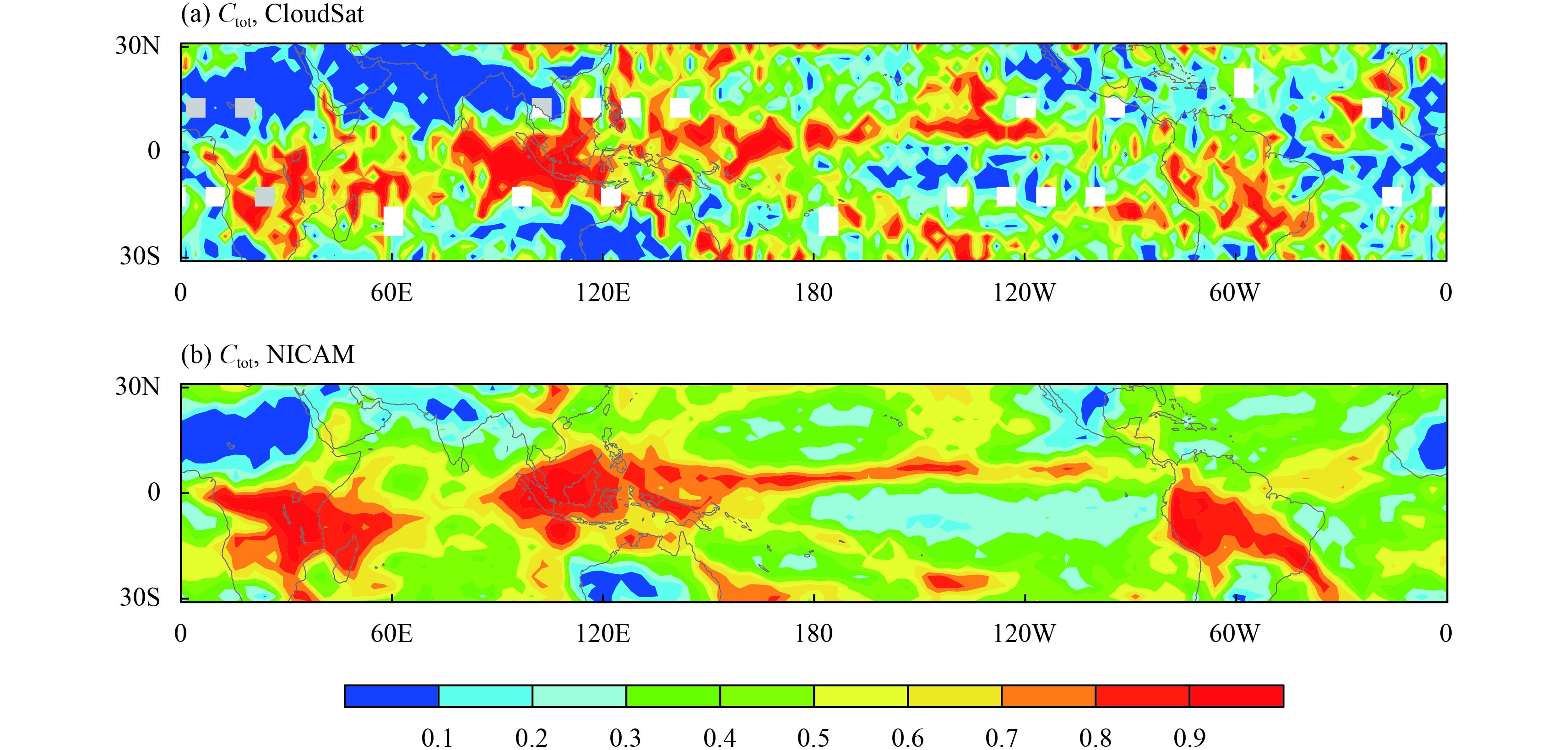
NICAM can be run using different horizontal resolutions depending on the grid division level used. In this study, data from a simulation using a grid division level of 11 (corresponding to a grid size of about 3.5 km) (Miura et al., 2007) are adopted; the cloud characteristics of this dataset have been extensively analyzed by Inoue et al. (2008, 2010), Masunaga et al. (2008), Sato et al. (2009), and Satoh et al. (2010). The simulation was started from 0000 UTC 25 December 2006 and integrated for 7 days. The results were stored as instantaneous snapshots at 0000 UTC on each day. Figures 1 and 2 show the simulated total cloud fraction and the zonal mean vertical cloud fraction profile, respectively, compared with those from the 2B-GEOPROF product of CloudSat observations (Marchand et al., 2008) during the same period. The NICAM simulation captures both the geographical distribution of cloud systems in the deep convective regions (Fig. 1) and the vertical cloud profiles in the tropics (Fig. 2). The cloud top height of NICAM in Fig. 2 is slightly higher than the CloudSat observations, which is because CloudSat does not detect optically thin clouds in the topmost layers (Stephens et al., 2008).
The variables used in this study are the mass mixing ratios of liquid and ice water condensates (qc and qi, respectively), in-cloud precipitation (qr) and snow (qs), and vertical velocity (w).
|
| Figure 1 Comparison of total cloud fraction (Ctot) between (a) CloudSat observations and (b) the NICAM simulation during the 7-day period starting from 0000 UTC 25 December 2006. |

|
| Figure 2 Comparison of zonal mean vertical cloud fraction profile between (a) CloudSat observations and (b) the NICAM simulation during the 7-day period starting from 0000 UTC 25 December 2006. |
To obtain Lcf at the resolution of the GCM and to establish the GCM-oriented relationship between Lcf and atmospheric convection, the original NICAM output is averaged based on a 2.8° × 2.8° (latitude × longitude) grid division, which is close to a T42 GCM resolution. The grid mean fields are then used to obtain Lcf using a stochastic cloud generator (Räisänen et al., 2004) as follows.
1) Diagnose the occurrence of cloud from qc, qi, qr, and qs. If qc + qi + qr + qs > 0.01 g kg –1 in a CRM grid cell, then this grid cell is regarded as cloudy (i.e., cloud fraction = 1), otherwise the grid cell is regarded as clear (i.e., cloud fraction = 0). This criterion was also used in Grabowski (1998).
2) Average the original CRM fields to the 2.8° × 2.8° grid division. The cloud fraction and the vertical velocity at 500 hPa (w500) are averaged within each GCM grid. These yield vertical distributions of cloud fractions and w500 for each GCM grid. In addition, the vertically projected cloud fraction (i.e., Ctot) for each GCM grid is derived by dividing the number of cloudy CRM columns by the total number of CRM columns within the grid.
3) Obtain Lcf. The vertical cloud fraction profile and Ctot in each GCM grid are supplied to the stochastic cloud generator with GenO incorporated to obtain Lcf. Lcf is defined as the value that gives the same Ctot as the original CRM cloud field when used in Eqs. (1) and (2). To demonstrate the effectiveness of using this procedure to capture the cloud overlap characteristics, a GCM grid with a typical cloud profile often seen in the tropical deep convective region is chosen as an example and the generated and original cloud structures are examined. The properties examined include the vertical cloud fraction profile, the downward cumulative cloud fraction, and the cloud fraction exposed to space at different heights (Fig. 3). It is suggested that, by applying the achieved Lcf in GenO, the generated cloud structures (dotted lines) resemble those of the original CRM field (solid lines). The characteristics of clouds shown in Fig. 3 are important to both solar reflectance and upward longwave emissivity. Therefore, the cloud structures generated by GenO with an accurate value of Lcf potentially facilitate the computation of radiation fields.

|
| Figure 3 Comparison of cloud features in a selected domain for the original CRM cloud field and that generated based on GenO with the true value of Lcf. (a) Cloud fraction at different altitudes, (b) downward cumulative cloud fraction, and (c) cloud fraction exposed to space at different altitudes. |
The vertical velocity in the mid-troposphere (w500) has been shown to be a representative indicator of tropical convection and cloud radiative forcing (Ichikawa et al., 2012). The relationship between Lcf and w500 is assessed in this subsection. As the overlap of clouds with very large or very small cloud fractions is of secondary importance for Ctot and radiation calculations, grids with maximum layer cloud fractions > 0.9 or < 0.1 are discarded.
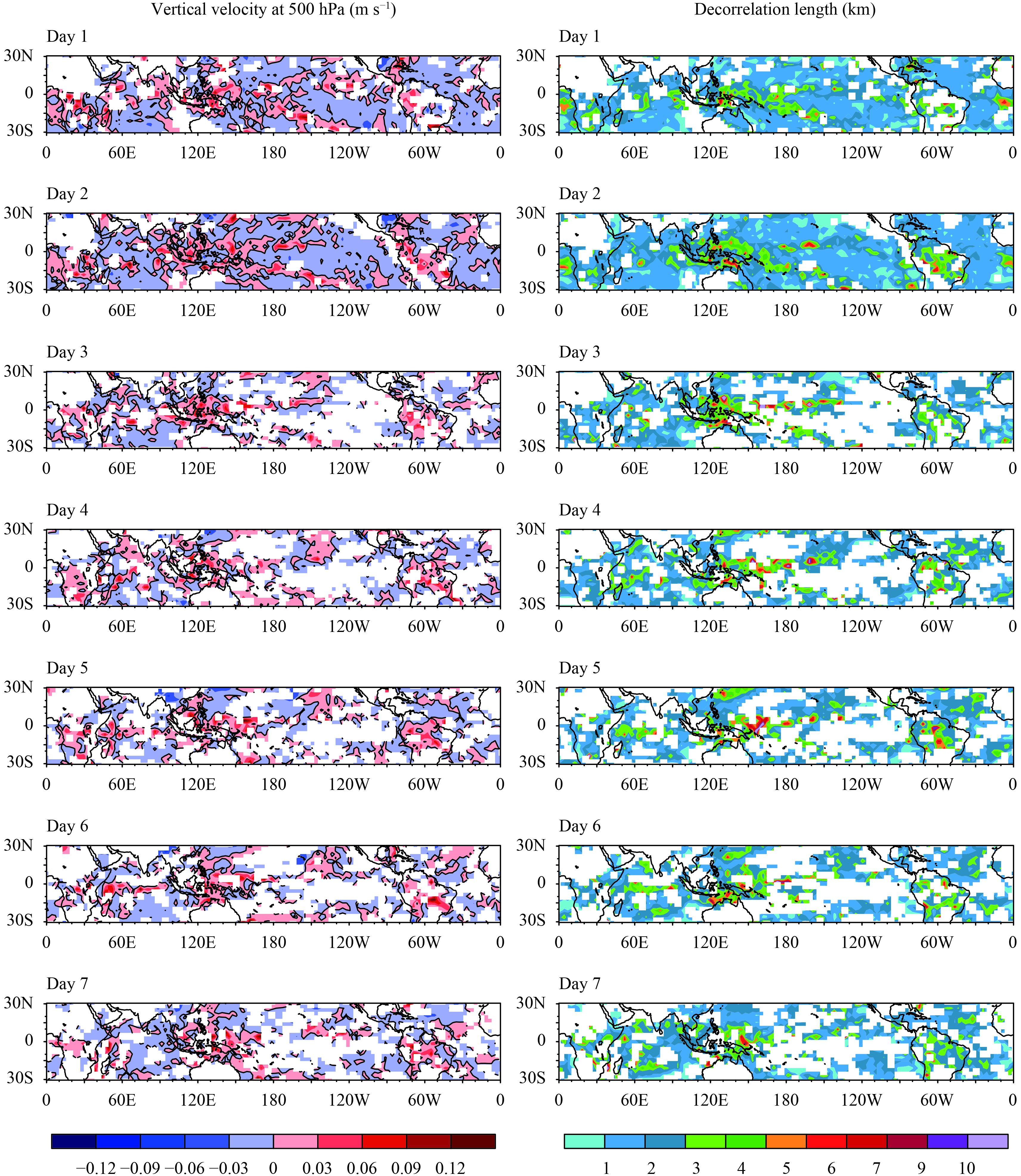
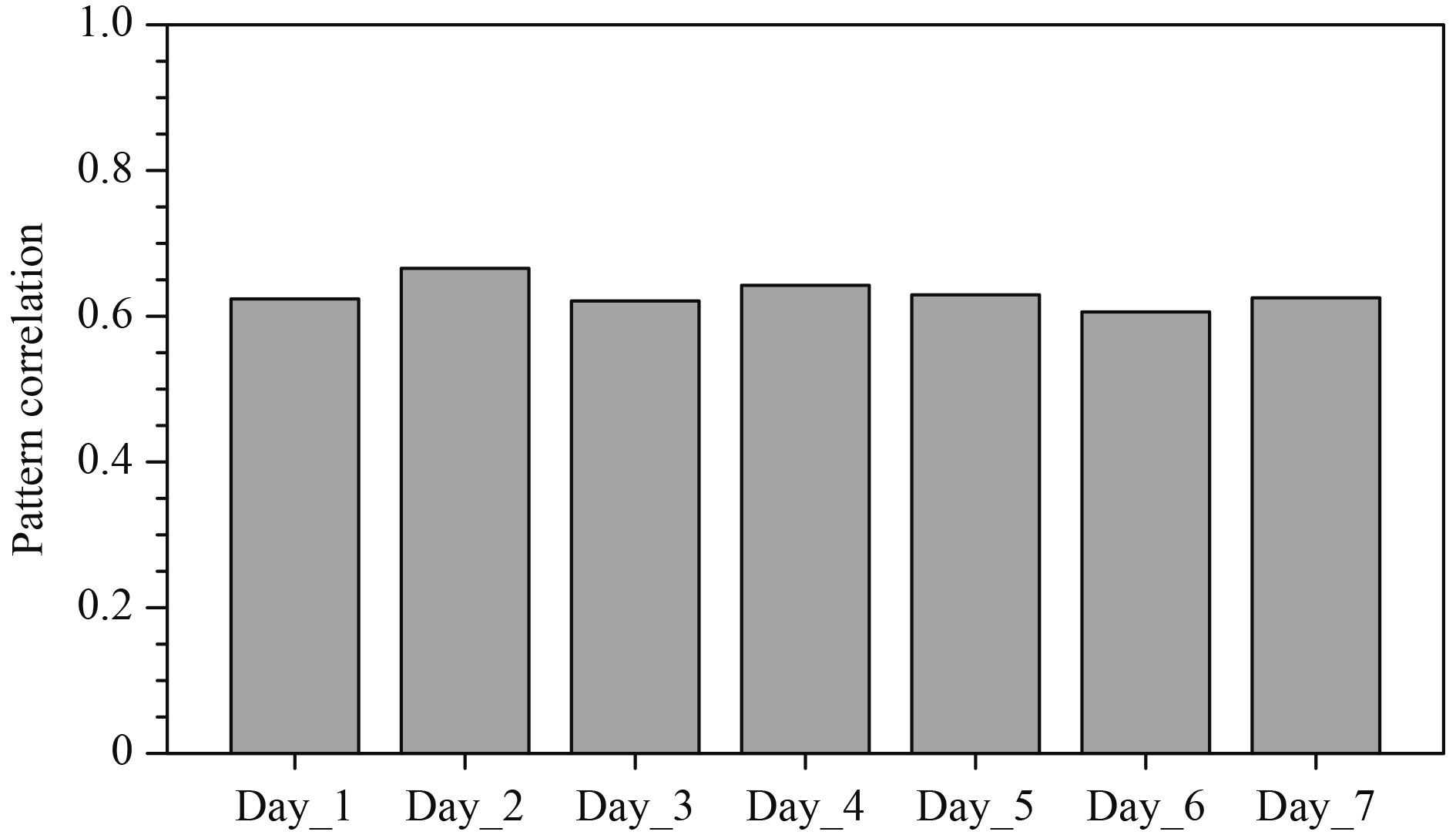
Figure 4 shows the distributions of Lcf and w500 for each model day. Domains with a large and positive w500 (e.g., the western Pacific and South America) mostly have a large value of Lcf (typically 4–7 km and up to 10 km in extreme cases). By contrast, in domains with a small or negative w500, Lcf is mostly about or below 2 km. Figure 5 shows the pattern correlation between the geographical distributions of Lcf and w500 for each snapshot. The pattern correlation stays at a moderate, but notable and constant level (from 0.61 to 0.66), implying a physically close association between Lcf and w500.
Based on pattern similarity and the clear difference between areas of ascent (w500 > 0) and descent ( w500 < 0), the relationship between Lcf and w500 will be explored separately for areas of ascent and descent.
|
| Figure 4 Distributions of w500 (left-hand panels) and Lcf (right-hand panels) in the tropics for each model day. Masked grids are those with maximum cloud fraction in the vertical direction of > 0.9 or < 0.1 and were thus eliminated from the analysis. |
|
| Figure 5 Pattern correlation between Lcf and w500 for each snapshot shown in Fig. 4. |
Figure 6 shows the statistics for Lcf and w500 and their relationships in the ascending areas. A total of 4926 samples were used to derive these statistics. The gray lines in Fig. 6a show the median and the first and third quartiles of Lcf for each bin of Lcf. These lines clearly show a positive relationship between Lcf and w500 for areas of ascent: when w500 < 0.02 m s –1, the most frequent occurrence of Lcf is around 2 km; as w500 increases to 0.08 m s–1, the corresponding value of Lcf increases to as much as 6–8 km, although the occurrence probability of w500 > 0.08 m s –1 is very small (Fig. 6b). Linear regression is conducted (as shown by the black solid line and the regression equation in Fig. 6a) for Lcf as a function of w500. The regression line captures very well the relationship illustrated by the yellow shaded area in Fig. 6a. The 95% confidence interval (blue dotted lines) and 95% prediction interval (red dashed lines) for this regression are also shown in Fig. 6a. The small 95% confidence interval (the mean of Lcf is 95% likely to fall into this interval for a given value of w500) suggests that the linear regression is an excellent representation of the average relationship between Lcf and w500; however, it should also be noted that the dispersion of the Lcf and w500 relationship is relatively large, as indicated by the 95% prediction interval (an individual Lcf for a given w500 falls into this interval with probability of 95%). The large dispersion of the Lcf and w500 relationship may stem primarily from the effect of other meteorological conditions on cloud overlap, which cannot be captured by a simple linear regression. Nevertheless, these results demonstrate that, in the statistical sense, Lcf and w500 are linearly related in the ascending regions of the tropics. The analysis in the following sections shows that addressing this statistical relationship will benefit the calculation of the cloud fraction and radiation fields.

|
| Figure 6 Statistics of Lcf and w500 constructed for the whole 7-day period. (a) The median (gray dashed line) and first and third quartiles (gray solid lines) of Lcf for each w500 bin (bin width 0.01 m s–1) and the linear regression of Lcf as a function of w500 (black solid line) (the linear regression equation and correlation coefficient are also shown). The yellow shaded area is the interquartile range of Lcf; the blue dotted line and red dashed line are the 95% confidence interval and 95% prediction interval of the regression, respectively. (b) Probability distribution function of w500. |
The same analysis for areas of descent shows that Lcf changes very little with w500 (data not shown) and that a value of 2 km is a good representation for these areas regardless of the specific w500. Consequently, Lcf can be approximated in the region 30°S–30°N depending on w500 as:
| ${L_{{\rm{cf}}}} = \left\{ \begin{array}{l}56.054 \times {w_{500}} + 1.951,\;\;\;{\rm{for}}\;\;{w_{500}} \geqslant 0.0,\\[8pt]2.0,\qquad \qquad \qquad \qquad {\rm{for}}\;\;{w_{500}} < 0.0.\end{array} \right.$ | (3) |
It should be noted that although GenO is independent of the vertical resolution, Eq. (3) may be affected by the vertical resolution of the NICAM data. Thus we should be cautious when applying Eq. (3) in a model with a notably different vertical resolution from that of NICAM, especially in the troposphere.
3.2 Evaluation in terms of cloud fractionThe better representation of Lcf is primarily expected to be capable of generating a realistic Ctot for given cloud fraction profiles. We evaluate here the generated Ctot by using the Lcf parameterized from Eq. (3) (denoted as PARA). Two other cloud overlap treatments are also included to compare with PARA: the traditional MRO assumption, which has been widely used not only in GCMs (Räisänen, 1998; Collins, 2001), but also in model assessment tools such as the CFMIP Observation Simulator Package (Bodas-Salcedo et al., 2011); and the simplified GenO using a constant Lcf (2 km) (denoted as G2KM), which applies the framework of GenO, but with a constant Lcf suggested as a global mean value (Barker, 2008). These cloud overlap treatments are used to generate sub-grid cloud fields from the cloud fraction profiles of the CRM and the values of Ctot of the generated fields are then compared with those of the original CRM fields.
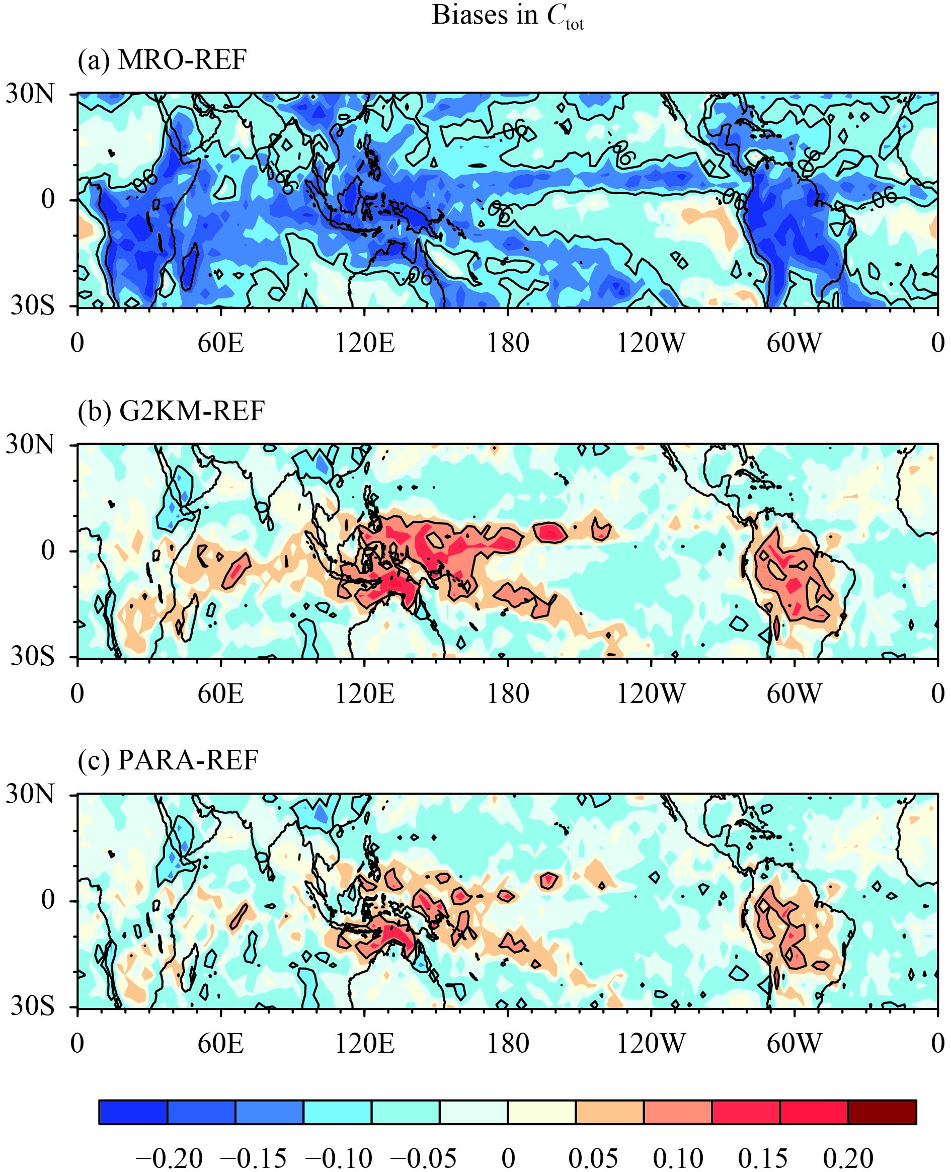
Figure 7 shows the 7-day mean biases of Ctot generated from the three cloud overlap representations relative to the reference value. It can be seen that the widely used MRO assumption remarkably underestimates Ctot in most regions. This is because there are few clear layers to separate the cloud layers in the vertical columns and therefore there is a maximum overlap of clouds in most cases. This demonstrates one drawback of the MRO technique: it depends greatly on the vertical resolution of the host model and is therefore usually non-equivalent among models.
The use of GenO significantly reduces the negative biases compared with the MRO assumption, even when a constant Lcf of 2 km is used (Fig. 7b). However, G2KM leads to notable Ctot biases in the ITCZ, especially in the western Pacific and Amazon regions, where clouds are generally more vertically organized because of systematic large-scale upward motion. When the dynamic representation of Lcf for regions of ascent is used, the cloud fraction errors in the ITCZ are remarkably reduced (Fig. 7c).
|
| Figure 7 Biases of generated Ctot using (a) the MRO assumption, (b) GenO with universal Lcf = 2 km (G2KM), and (c) GenO with dynamic representation of Lcf (PARA) relative to the true Ctot from the CRM (REF). Contour lines are shown for ±0.06. |
Radiation calculations are performed for the generated cloud fields and the original CRM cloud fields in the evaluation using the BCC–RAD correlated-k distribution radiation model (Zhang et al., 2003, 2006a, b ), which has been implemented in the GCM of the Beijing Climate Center (BCC_AGCM2.0.1) (Zhang et al., 2014). For both the generated and original cloud fields, the cloud water/ice content in each GCM grid is obtained as a grid mean value to eliminate the effect of the horizontal distributions of cloud water/ice. Because only the cloud and dynamic output from NICAM are stored (due to the large amount of data), we apply in the radiation calculation the atmospheric pressures, temperatures, and gas concentrations from the tropical atmosphere of the US Air Force Geophysics Laboratory atmospheric models (Anderson et al., 1986) and the broadband surface albedos for the ocean (0.08, Jin et al., 2004) and solid surfaces (0.28, Liang, 2001), respectively.
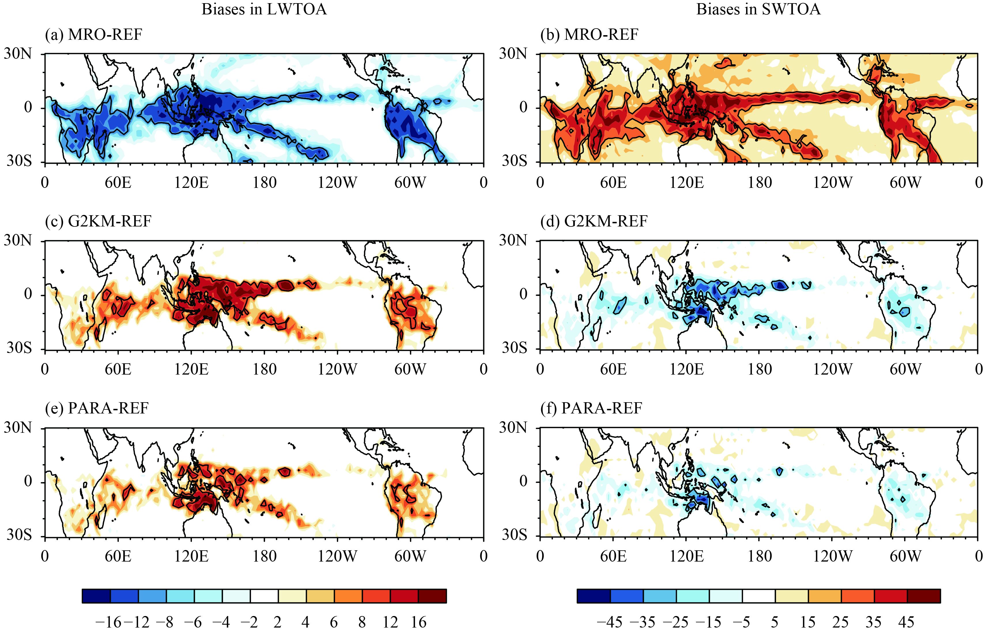
Figure 8 shows the biases in the generated net longwave (LWTOA) and shortwave (SWTOA) radiative fluxes at the top of the atmosphere relative to the CRM results. The largest radiation biases occur in the ITCZ, where the largest Ctot biases are also seen. The MRO assumption shows significant negative biases for LWTOA and positive biases for SWTOA (mostly > 10 and > 25 W m –2, respectively) (Figs. 8a, b) due to the underestimation of Ctot. Figures 8c and 8d show that the use of GenO with a constant Lcf of 2 km reduces the biases in subtropical regions, but also introduces notable biases in the ITCZ with opposite signs to the biases of the MRO assumption. The dynamic representation of Lcf largely reduces the negative biases in the ITCZ (Figs. 8e, f), with considerably fewer regions having absolute biases > 10 and > 25 W m –2 for LWTOA and SWTOA, respectively.
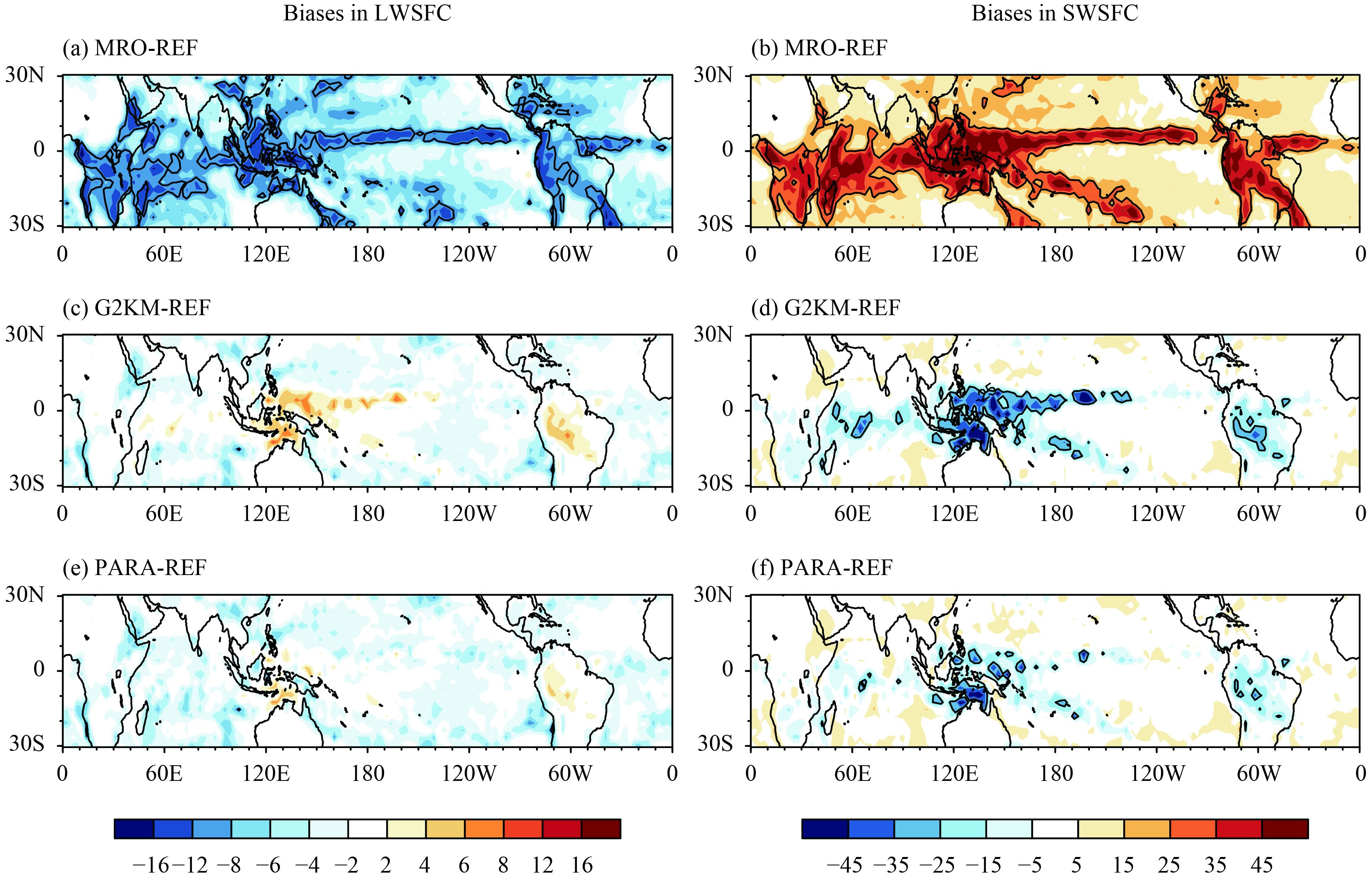
Figure 9 shows the biases in the net longwave (LWSFC) and shortwave (SWSFC) radiative fluxes at the surface. By comparing Fig. 9 with Fig. 8, it is seen that the main features of the biases at the surface are similar to those at the TOA, except that G2KM and PARA have much smaller (larger) biases in LWSFC over (outside) the ITCZ. PARA has the smallest errors among the three treatments of cloud overlap over the ITCZ for both LWSFC and SWSFC. It is therefore evident that the dynamic representation of Lcf yields the best spatial patterns of the radiation fields.
|
| Figure 8 Biases of generated LWTOA (left-hand panels) and SWTOA (right-hand panels) using (a, b) the MRO assumption, (c, d) GenO with Lcf = 2 km universally, and (e, f) GenO with dynamic representation of Lcf, relative to those calculated directly from the CRM fields. The downward direction is defined as positive. The contour lines for ±10 and ±25 W m–2 are shown for LWTOA and SWTOA, respectively. |
|
| Figure 9 As in Fig. 8, but for (a, c, e) LWSFC and (b, d, f) SWSFC. |
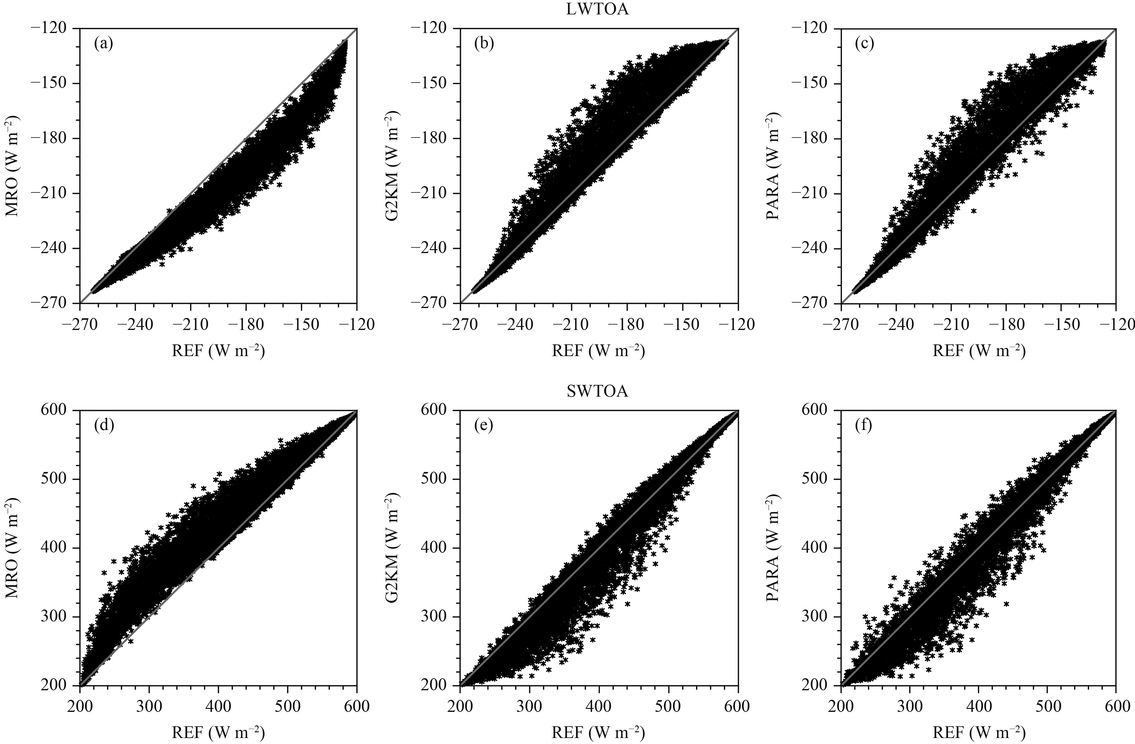
Figures 10 and 11 are scatter diagrams comparing the generated and reference radiation fields at the TOA and surface, respectively. Systematically negative biases in LWTOA and positive biases in SWTOA are shown for the MRO assumption (Figs. 10a, d) and the opposite for G2KM (Figs. 10b, e). PARA shows little systematic bias in LWTOA and SWTOA—that is, the points are distributed more symmetrically around the reference lines (Figs. 10c, f). Similar features are also shown at the surface (Fig. 11), except that G2KM and PARA resemble each other for the LWSFC (Figs. 11b, c), consistent with their similarity in Fig. 9.
Figure 12 shows the tropical-averaged radiation biases for all areas (solid fill) and areas of ascent only (hatched fill). As expected, the MRO assumption shows the largest errors relative to the reference, especially for the shortwave fluxes (about 16 W m–2 at both the TOA and the surface). G2KM performs much better than the MRO assumption, with absolute errors of approximately 2 W m–2 for LWTOA and SWTOA. PARA reduces the errors more significantly, especially for shortwave fluxes. The error in LWSFC of PARA is more negative than that of G2KM (Fig. 12c); this is because PARA reduces the positive errors in the ITCZ (as shown in Fig. 9) that compensate for negative errors in other regions. It should be stressed that, for most of these variables, PARA reduces the all-area mean errors as effectively as it does in the areas of ascent only, implying that unrealistic cloud overlap treatment in areas of ascent is a major source of radiation error in tropical areas. Considering that these areas typically have large radiation biases in GCM simulations (Lauer and Hamilton, 2013), the introduction of PARA-like overlap treatment could possibly reduce the uncertainty in tropical radiation calculations.
|
| Figure 10 Comparisons between LWTOA and SWTOA calculated from generated cloud fields with different cloud overlap treatments (MRO, G2KM, and PARA) and the values calculated directly from the CRM fields (REF) for the tropical areas. |

|
| Figure 11 As in Fig. 10, but for (a, b, c) LWSFC and (d, e, f) SWSFC. |

|
| Figure 12 Tropical mean biases in (a) LWTOA, (b) SWTOA, (c) LWSFC, and (d) SWSFC for generated clouds fields with different cloud overlap treatments (MRO, G2KM, and PARA) compared with those for the CRM fields (REF) over all areas (solid fill) and areas of ascent only (hatched fill). |
The treatment of vertical cloud overlap also influences the radiative heating rate in the atmosphere, a property important for atmospheric stability and circulation. Figure 13 compares the effects of different overlap treatments on the ascending area mean longwave (LWHTR) and shortwave (SWHTR) heating rates. The LWHTRs of different overlap treatments are similar to each other in the middle to higher troposphere, but near the surface the MRO assumption shows remarkable longwave cooling (Fig. 13b) and G2KM and PARA show overestimated longwave heating. This is probably due to the underestimated (overestimated) cloud fraction of the MRO assumption (G2KM and PARA) over these regions (as shown in Fig. 7). For the SWHTR, the MRO assumption underestimates heating around altitudes of 2 and 10 km, whereas G2KM overestimates heating around 10 km height and underestimates heating in the lower troposphere. PARA has a similar SWHTR to G2KM, but the bias in the upper troposphere is remarkably reduced and the bias in the lower troposphere is also reduced to some extent. These changes in the radiative heating rates caused by applying PARA, when coupled with a circulation model, will exert an influence on atmospheric stability in the vertical direction and consequently change the dynamic circulation. These aspects will be explored in future studies.

|
| Figure 13 (a) Longwave and (c) shortwave heating rates for the three cloud overlap treatments (MRO, G2KM, and PARA) and REF over the tropical ascending area and the differences between the three overlap treatments and REF (b and d, respectively). |
The treatment of cloud overlap plays a crucial part in radiation calculations in GCMs. However, it is difficult to achieve a unified description of this highly variable (both spatially and temporally) property of clouds. By using the simulation of a CRM isolated to the tropical region, a statistical relationship between cloud overlap and convective strength was found and a dynamic representation of Lcf (which determines the extent of cloud overlap) was established. A simple linear regression of Lcf as a function of vertical velocity in the mid-troposphere is capable of partly capturing the cloud overlap dynamic connection and thus remarkably reduces biases in the cloud fraction and radiation fields in tropical convective regions. These regions are where major cloud fraction and radiation biases exist and therefore a reduction in these biases would make a significant contribution to the reduction of the overall bias in the tropics.
In spite of the improvement in cloud fraction and radiation fields by implementing the convection-dependent overlap treatment, the results rely on the fidelity of the intrinsic physical and dynamic properties of the CRM. Cloud overlap characteristics also depend on other meteorological conditions in addition to convection, such as wind shear and atmospheric instability (Naud et al., 2008; Di Giuseppe and Tompkins, 2015), even in the tropical deep convection region. Thus the method derived here should not be regarded as a perfect deterministic relationship between cloud overlap and convection, but an empirical, statistical approximation of the contribution of convection to cloud overlap. Other meteorological conditions are virtually ignored in the overlap treatment in this study. The treatment of cloud overlap in extratropical areas was not addressed in this work because the overlap of clouds in such areas relates to large-scale meteorological conditions in a more complex manner than in the tropics. Another aspect of sub-grid cloud structures, i.e., the horizontally inhomogeneous distribution of cloud water, is also highly important in radiation calculations (Barker et al., 1996; Wu and Liang, 2005a); this aspect was excluded in the overlap treatment of this study.
The results of this study do, however, provide modelers with a simple and effective approach to more realistically address cloud overlap in tropical regions. This approach acts as another, although not perfect, constraint of cloud–radiation interactions, an aspect of GCMs that contributes greatly to uncertainties in simulations. The form of the Lcf–convection relationship is open to further improvement and the application of this method to extended CRM and observational datasets (e.g., datasets from the multi-sensor A-Train constellation) will provide essential evidence of the Lcf–convection relationship from the points of view of both simulation and observation, and produce more robust treatments of Lcf in future studies.
| Anderson, G. P., S. A. Clough, F. X. Kneizys, et al., 1986: AFGL atmospheric constituent profiles (0.120 km). AFGL Tech. Rep., AFGL-TR-86-0110, Bedford, MA, Air Force Geophys. Lab., 1–43. |
| Barker, H. W., 2008: Representing cloud overlap with an effective decorrelation length: An assessment using CloudSat and CALIPSO data. J. Geophys. Res., 113, D24205. DOI:10.1029/2008JD010391 |
| Barker, H. W., and P. Räisänen, 2005: Radiative sensitivities for cloud structural properties that are unresolved by conventional GCMs. Quart. J. Roy. Meteor. Soc., 131, 3103–3122. DOI:10.1256/qj.04.174 |
| Barker, H. W., B. A. Wiellicki, and L. Parker, 1996: A parameterization for computing grid-averaged solar fluxes for inhomogeneous marine boundary layer clouds. Part II: Validation using satellite data. J. Atmos. Sci., 53, 2304–2316. DOI:10.1175/1520-0469(1996)053<2304:APFCGA>2.0.CO;2 |
| Barker, H. W., G. L. Stephens, P. Partain, et al., 2003: Assessing 1D atmospheric solar radiative transfer models: Interpretation and handling of unresolved clouds. J. Climate, 16, 2676–2699. DOI:10.1175/1520-0442(2003)016<2676:ADASRT>2.0.CO;2 |
| Bergman, J. W., and P. J. Rasch, 2002: Parameterizing vertically coherent cloud distributions. J. Atmos. Sci., 59, 2165–2182. DOI:10.1175/1520-0469(2002)059<2165:PVCCD>2.0.CO;2 |
| Bodas-Salcedo, A., M. J. Webb, S. Bony, et al., 2011: COSP: Satellite simulation software for model assessment. Bull. Am. Meteor. Soc., 92, 1023–1043. DOI:10.1175/2011BAMS2856.1 |
| Bony, S., K.-M. Lau, and Y. C. Sud, 1997: Sea surface temperature and large-scale circulation influences on tropical greenhouse effect and cloud radiative forcing. J. Climate, 10, 2055–2077. DOI:10.1175/1520-0442(1997)010<2055:SSTALS>2.0.CO;2 |
| Bony, S., B. Stevens, D. M. W. Frierson, et al., 2015: Clouds, circulation and climate sensitivity. Nature Geosci., 8, 261–268. DOI:10.1038/ngeo2398 |
| Collins, W. D., 2001: Parameterization of generalized cloud overlap for radiative calculations in general circulation models. J. Atmos. Sci., 58, 3224–3242. DOI:10.1175/1520-0469(2001)058<3224:POGCOF>2.0.CO;2 |
| Di Giuseppe, F., 2005: Sensitivity of one-dimensional radiative biases to vertical cloud-structure assumptions: Validation with aircraft data. Quart. J. Roy. Meteor. Soc., 131, 1655–1676. DOI:10.1256/qj.03.129 |
| Di Giuseppe, F., and A. M. Tompkins, 2015: Generalizing cloud overlap treatment to include the effect of wind shear. J. Atmos. Sci., 72, 2865–2876. DOI:10.1175/JAS-D-14-0277.1 |
| GEWEX Cloud System Science Team, 1993: The GEWEX cloud system study (GCSS). Bull. Amer. Meteor. Soc., 74, 387–400. DOI:10.1175/1520-0477(1993)074<0387:TGCSS>2.0.CO;2 |
| Grabowski, W. W., 1998: Toward cloud resolving modeling of large-scale tropical circulations: A simple cloud microphysics parameterization. J. Atmos. Sci., 55, 3283–3298. DOI:10.1175/1520-0469(1998)055<3283:TCRMOL>2.0.CO;2 |
| Hogan, R. J., and A. J. Illingworth, 2000: Deriving cloud overlap statistics from radar. Quart. J. Roy. Meteor. Soc., 126, 2903–2909. DOI:10.1002/qj.49712656914 |
| Ichikawa, H., H. Masunaga, Y. Tsushima, et al., 2012: Reproducibility by climate models of cloud radiative forcing associated with tropical convection. J. Climate, 25, 1247–1262. DOI:10.1175/JCLI-D-11-00114.1 |
| Inoue, T., M. Satoh, H. Miura, et al., 2008: Characteristics of cloud size of deep convection simulated by a global cloud resolving model over the western tropical Pacific. J. Meteor. Soc. Japan, 86A, 1–15. DOI:10.2151/jmsj.86A.1 |
| Inoue, T., M. Satoh, Y. Hagihara, et al., 2010: Comparison of high-level clouds represented in a global cloud system-resolving model with CALIPSO/CloudSat and geostationary satellite observations. J. Geophys. Res., 115, D00H22. DOI:10.1029/2009JD012371 |
| Jin, Z. H., T. P. Charlock, W. L. Jr. Smith, et al., 2004: A parameterization of ocean surface albedo. Geophys. Res. Lett., 31, L22301. DOI:10.1029/2004GL021180 |
| Jing, X. W., H. Zhang, J. Peng, et al., 2016: Cloud overlapping parameter obtained from CloudSat/CALIPSO dataset and its application in AGCM with McICA scheme. Atmos. Res., 170, 52–65. DOI:10.1016/j.atmosres.2015.11.007 |
| Kato, S., S. Sun-Mack, M. F. Miller, et al., 2010: Relationships among cloud occurrence frequency, overlap, and effective thickness derived from CALIPSO and CloudSat merged cloud vertical profiles. J. Geophys. Res., 115, D00H28. DOI:10.1029/2009JD012277 |
| Lauer, A., and K. Hamilton, 2013: Simulating clouds with global climate models: A comparison of CMIP5 results with CMIP3 and satellite data. J. Climate, 26, 3823–3845. DOI:10.1175/JCLI-D-12-00451.1 |
| Li, J., J. Huang, K. Stamnes, et al., 2015: A global survey of cloud overlap based on CALIPSO and CloudSat measurements. Atmos. Chem. Phys., 15, 519–536. DOI:10.5194/acp-15-519-2015 |
| Li, J. D., Y. M. Liu, and G. X. Wu, 2009: Cloud radiative forcing in Asian monsoon region simulated by IPCC AR4 AMIP models. Adv. Atmos. Sci., 26, 923–939. DOI:10.1007/s00376-009-8111-x |
| Liang, S. L., 2001: Narrowband to broadband conversions of land surface albedo. I: Algorithms. Remote Sens. Environ., 76, 213–238. DOI:10.1016/S0034-4257(00)00205-4 |
| Liang, X. Z., and W. C. Wang, 1997: Cloud overlap effects on general circulation model climate simulations. J. Geophys. Res., 102, 11039–11047. DOI:10.1029/97JD00630 |
| Liang, X. Z., and X. Q. Wu, 2005: Evaluation of a GCM subgrid cloud-radiation interaction parameterization using cloud-resolving model simulations. Geophys. Res. Lett., 32, L06801. DOI:10.1029/2004GL022301 |
| Mace, G. G., and S. Benson-Troth, 2002: Cloud-layer overlap characteristics derived from long-term cloud radar data. J. Climate, 15, 2505–2515. DOI:10.1175/1520-0442(2002)015<2505:CLOCDF>2.0.CO;2 |
| Marchand, R., G. G. Mace, T. Ackerman, et al., 2008: Hydrometeor detection using CloudSat—An earth-orbiting 94-GHz cloud radar . J. Atmos. Oceanic Technol., 25, 519–533. DOI:10.1175/2007JTECHA1006.1 |
| Masunaga, H., M. Satoh, and H. Miura, 2008: A joint satellite and global cloud-resolving model analysis of a Madden–Julian Oscillation event: Model diagnosis.. J. Geophys. Res., 113, D17210. DOI:10.1029/2008JD009986 |
| Miura, H., M. Satoh, T. Nasuno, et al., 2007: A Madden–Julian oscillation event realistically simulated by a global cloud-resolving model. Science, 318, 1763–1765. DOI:10.1126/science.1148443 |
| Morcrette, J. J., and Y. Fouquart, 1986: The overlapping of cloud layers in shortwave radiation parameterizations. J. Atmos. Sci., 43, 321–328. DOI:10.1175/1520-0469(1986)043<0321:TOOCLI>2.0.CO;2 |
| Nakanishi, M., and H. Niino, 2006: An improved Mellor-Yamada level-3 model: Its numerical stability and application to a regional prediction of advection fog. Bound.-Layer Meteor., 119, 397–407. DOI:10.1007/s10546-005-9030-8 |
| Naud, C. M., A. Del Genio, G. G. Mace, et al., 2008: Impact of dynamics and atmospheric state on cloud vertical overlap. J. Climate, 21, 1758–1770. DOI:10.1175/2007JCLI1828.1 |
| Oreopoulos, L., and M. Khairoutdinov, 2003: Overlap properties of clouds generated by a cloud-resolving model. J. Geophys. Res., 108, 4479. DOI:10.1029/2002JD003329 |
| Oreopoulos, L., D. Lee, Y. C. Sud, et al., 2012: Radiative impacts of cloud heterogeneity and overlap in an atmospheric general circulation model. Atmos. Chem. Phys., 12, 9097–9111. DOI:10.5194/acp-12-9097-2012 |
| Peng, J., H. Zhang, and X. Y. Shen, 2013: Analysis of vertical structure of clouds in East Asia with CloudSat data. Chinese J. Atmos. Sci., 37, 91–100. DOI:10.3878/j.issn.1006-9895.2012.11188 |
| Räisänen, P., 1998: Effective longwave cloud fraction and maximum-random overlap of clouds: A problem and a solution. Mon. Wea. Rev., 126, 3336–3340. DOI:10.1175/1520-0493(1998)126<3336:ELCFAM>2.0.CO;2 |
| Räisänen, P., H. W. Barker, M. F. Khairoutdinov, et al., 2004: Stochastic generation of subgrid-scale cloudy columns for large-scale models. Quart. J. Roy. Meteor. Soc., 130, 2047–2067. DOI:10.1256/qj.03.99 |
| Randall, D., M. Khairoutdinov, A. Arakawa, et al., 2003: Breaking the cloud parameterization deadlock. Bull. Amer. Meteor. Soc., 84, 1547–1564. DOI:10.1175/BAMS-84-11-1547 |
| Sato, T., H. Miura, M. Satoh, et al., 2009: Diurnal cycle of precipitation in the tropics simulated in a global cloud-resolving model. J. Climate, 22, 4809–4826. DOI:10.1175/2009JCLI2890.1 |
| Satoh, M., T. Matsuno, H. Tomita, et al., 2008: Nonhydrostatic icosahedral atmospheric model (NICAM) for global cloud resolving simulations. J. Comput. Phys., 227, 3486–3514. DOI:10.1016/j.jcp.2007.02.006 |
| Satoh, M., T. Inoue, and H. Miura, 2010: Evaluations of cloud properties of global and local cloud system resolving models using CALIPSO and CloudSat simulators. J. Geophys. Res., 115, D00H14. DOI:10.1029/2009JD012247 |
| Satoh, M., H. Tomita, H. Yashiro, et al., 2014: The non-hydrostatic icosahedral atmospheric model: Description and development. Progress in Earth and Planetary Science, 1, 18. DOI:10.1186/s40645-014-0018-1 |
| Shonk, J. K. P., R. J. Hogan, J. M. Edwards, et al., 2010: Effect of improving representation of horizontal and vertical cloud structure on the Earth’s global radiation budget. Part I: Review and parametrization. Quart. J. Roy. Meteor. Soc., 136, 1191–1204. DOI:10.1002/qj.647 |
| Stephens, G. L., 2005: Cloud feedbacks in the climate system: A critical review. J. Climate, 18, 237–273. DOI:10.1175/JCLI-3243.1 |
| Stephens, G. L., D. G. Vane, S. Tanelli, et al., 2008: CloudSat mission: Performance and early science after the first year of operation. J. Geophys. Res., 113, D00A18. DOI:10.1029/2008JD009982 |
| Tian, L., and J. A. Curry, 1989: Cloud overlap statistics. J. Geophys. Res., 94, 9925–9935. DOI:10.1029/JD094iD07p09925 |
| Tomita, H., and M. Satoh, 2004: A new dynamical framework of nonhydrostatic global model using the icosahedral grid. Fluid Dyn. Res., 34, 357–400. DOI:10.1016/j.fluiddyn.2004.03.003 |
| Tompkins, A. M., and F. Di Giuseppe, 2015: An interpretation of cloud overlap statistics. J. Atmos. Sci., 72, 2877–2889. DOI:10.1175/JAS-D-14-0278.1 |
| Wang, X. C., Y. M. Liu, and Q. Bao, 2016: Impacts of cloud overlap assumptions on radiative budgets and heating fields in convective regions. Atmos. Res., 167, 89–99. DOI:10.1016/j.atmosres.2015.07.017 |
| Wu, X. Q., and X.-Z. Liang, 2005a: Radiative effects of cloud horizontal inhomogeneity and vertical overlap identified from a monthlong cloud-resolving model simulation. J. Atmos. Sci., 62, 4105–4112. DOI:10.1175/JAS3565.1 |
| Wu, X. Q., and X.-Z. Liang, 2005b: Effect of subgrid cloud-radiation interaction on climate simulations. Geophys. Res. Lett., 32, L24806. DOI:10.1029/2005GL024432 |
| Wu, X. Q., and X. F. Li, 2008: A review of cloud-resolving model studies of convective processes. Adv. Atmos. Sci., 25, 202–212. DOI:10.1007/s00376-008-0202-6 |
| Zhang, F., X.-Z. Liang, J. N. Li, et al., 2013: Dominant roles of subgrid-scale cloud structures in model diversity of cloud radiative effects. J. Geophys. Res. Atmos., 118, 7733–7749. DOI:10.1002/jgrd.50604 |
| Zhang, H., and X. W. Jing, 2010: Effect of cloud overlap assumptions in climate models on modeled earth–atmosphere radiative fields. Chinese J. Atmos. Sci., 34, 520–532. DOI:10.3878/j.issn.1006-9895.2010.03.06 |
| Zhang, H., and X. W. Jing, 2016: Advances in studies of cloud overlap and its radiative transfer in climate models. J. Meteor. Res., 30, 156–168. DOI:10.1007/s13351-016-5164-5 |
| Zhang, H., T. Nakajima, G. Y. Shi, et al., 2003: An optimal approach to overlapping bands with correlated k distribution method and its application to radiative calculations . J. Geophys. Res., 108, 4641. DOI:10.1029/2002JD003358 |
| Zhang, H., G. Y. Shi, T. Nakajima, et al., 2006a: The effects of the choice of the k-interval number on radiative calculations . J. Quant. Spectro. Rad. Trans., 98, 31–43. DOI:10.1016/j.jqsrt.2005.05.090 |
| Zhang, H., T. Suzuki, T. Nakajima, et al., 2006b: Effects of band division on radiative calculations. Opt. Eng., 45, 016002. DOI:10.1117/1.2160521 |
| Zhang, H., J. Peng, X. W. Jing, et al., 2013: The features of cloud overlapping in eastern Asia and their effect on cloud radiative forcing. Sci. China Earth Sci., 56, 737–747. DOI:10.1007/s11430-012-4489-x |
| Zhang, H., X. Jing, and J. Li, 2014: Application and evaluation of a new radiation code under McICA scheme in BCC_AGCM2.0.1. Geosci. Model Dev., 7, 737–754. DOI:10.5194/gmd-7-737-2014 |
 2018, Vol. 32


