The Chinese Meteorological Society
Article Information
- Wang, C. X., and Z. F. Ma, 2018.
- Quasi-3-yr Cycle of Rainy Season Precipitation in Tibet Related to Different Types of ENSO during 1981–2015. 2018.
- J. Meteor. Res., 32(2): 181-190
- http://dx.doi.org/10.1007/s13351-018-7100-3
Article History
- Received July 11, 2017
- in final form November 8, 2017
2. Key Laboratory of Sichuan Province for Heavy Rain and Drought–Flood Disasters in Plateau and Basin, Chengdu 610072
The Qinghai–Tibetan Plateau has important dynamic and thermodynamic effects on the regional and global weather and climate. These effects have been investigated through field experiments, data analyses, and theoretical investigations (Tao and Ding, 1981; Ye, 1981; Zheng and Liou, 1986; Yanai et al., 1992; Wu and Liu, 2016), but studies focusing on the climatic variability of the Tibetan Plateau itself have been relatively limited.
Tibet is the main part of the Qinghai–Tibetan Plateau, the climate of which is mainly controlled by the South Asian summer monsoon (SASM). There is a strong correlation between the rainy season precipitation in Tibet (RSPT) and the annual precipitation (Lu et al., 2008). Liu and Yin (2001) showed that the dominant spatial pattern of the interannual variability of summer precipitation was a seesaw structure between the southern and northern parts of the eastern Qinghai–Tibetan Plateau and that pattern was closely associated with the North Atlantic Oscillation. Zhou et al. (2000) reported that the RSPT shows a quasi-3-yr cycle that can be divided into three categories: (1) the same anomalies over the whole region; (2) a north–south reverse pattern; and (3) an east–west reverse pattern. The annual precipitation in most areas of Tibet shows an increasing trend, but the Ali Region has the opposite trend (Du and Ma, 2004). Huang et al. (2013) reported that precipitation in Tibet has a developing trend toward unbalanced and extreme events.
The El Niño–Southern Oscillation (ENSO) is consi-dered to be the strongest climate signal and is the key factor affecting summer droughts and floods in China. There is usually more precipitation in the Yangtze River region in the year following an El Niño event and less precipitation in the Huaihe basin; the opposite is seen during a La Niña event (Jin and Tao, 1999). Pubu et al. (2002) investigated the relationship between the RSPT and ENSO events and found that the most serious droughts tend to occur in El Niño years, whereas severe floods often occur in La Niña years. There are two basic types of El Niño—eastern Pacific (EP) events and central Pacific (CP) events—distinguished in the warming region of the equatorial Pacific (Fu and Fletcher, 1985). The frequency of CP El Niño events began to increase significantly after the 1990s (Yeh et al., 2009). Kug et al. (2009) proposed that the two ENSO events had different physical mechanisms and that the circulation anomalies and climate effects were also different. The EP (CP) type of El Niño is linked to an anomalous positive/negative/ positive (negative/positive/negative) rainfall pattern over East Asia and the equatorial Pacific (Yuan and Yang, 2012).
There have been few reported studies on the effect of different types of ENSO on the RSPT. As ENSO is an important climate signal, an in-depth analysis of the relationship between different types of ENSO and the RSPT will enhance our understanding of rainfall mechanisms in the rainy season in Tibet and improve the climate prediction for this region. In this study, we will analyze the evolution of the quasi-3-yr cycle of the RSPT, investigate its synergetic relationship to different types of ENSO, and propose possible mechanisms for the relationship.
2 Data and methodology 2.1 DataThe main datasets used in this paper include: (1) daily precipitation data from 38 meteorological stations in Tibet from 1 May to 30 September (the flood season) during 1981–2015; (2) the monthly mean NOAA Extended Reconstructed Sea Surface Temperature dataset, version 4, gridded at 2° × 2° resolution (www.esrl.noaa.gov/ psd/data/gridded/data.noaa.ersst.v4.html); and (3) the monthly mean horizontal winds, omega, geopotential height, and specific humidity data from 100 to 1000 hPa, gridded at 2.5° × 2.5° resolution from the NCEP/NCAR reanalysis 1 dataset (www.esrl.noaa.gov/psd/data/gridded/data.ncep.reanalysis.pressure.html).
2.2 MethodologyThe multi-taper method with singular value decomposition (MTM-SVD) is a multivariable frequency domain decomposition technique proposed by Mann and Park (1994). The detection of the climate signal is a combination of an MTM of spectral analysis and an SVD method for variable fields. The MTM-SVD method has been widely used in meteorological research (Minobe, 2000; Han et al., 2008; Small and Islam, 2008; Apipattanavis et al., 2009). Mann and Park (1994, 1996, 1999) carried out much research on climate signal tests and found that this method has many advantages over general analysis, wavelet analysis, and SVD signal detection methods: (1) the objects of analysis in the MTM-SVD method can be multidimensional or multi-site climate variables and raw meteorological data can be used; (2) the MTM method can effectively prevent spectral leakage; (3) the localized fractional variance (LFV) spectrum is an effective parameter for detecting signals in the frequency domain and the peaks at a given frequency indicate a potentially important spatiotemporal signal; (4) spatiotemporal signals can be reconstructed that can more directly analyze and describe the temporal and spatial evolution and processes of vibration on different timescales; and (5) the MTM-SVD technology can be extended to the coupled region, so that more than one region can be analyzed at the same time.
An outline of the method is given here; a more detailed description is given in Mann and Park (1996, 1999) and the specific analysis routines are freely available online (http://www.meteo.psu.edu/;mann/Mann/ tools/tools.html).
2.2.1 Signal detectionThe time series
| ${ Y}\left( {{f_0}} \right) = \left[ \begin{array}{l}Y_1^1\left( {{f_0}} \right)Y_1^2\left( {{f_0}} \right) \cdot \cdot \cdot Y_1^S\left( {{f_0}} \right)\\[7pt]Y_2^1\left( {{f_0}} \right)Y_2^2\left( {{f_0}} \right) \cdot \cdot \cdot Y_2^S\left( {{f_0}} \right)\\[7pt] \cdot \cdot \cdot \\[7pt]Y_M^1\left( {{f_0}} \right)Y_M^2\left( {{f_0}} \right) \cdot \cdot \cdot Y_M^S\left( {{f_0}} \right)\end{array} \right],$ | (1) |
| ${ Y}\left( {{f_0}} \right) = { U}\left( {{f_0}} \right)\cdot { L}\left( {{f_0}} \right)\cdot {{ V}^ + }\left( {{f_0}} \right).\qquad \quad\,\,$ | (2) |
A complex SVD is then computed on each matrix
| ${ Y}_m^{\rm{s}}\left( {{f_0}} \right) = \sum\limits_{k = 1}^K {{ U}_m^k\left( {{f_0}} \right)} {\gamma _k}\left( {{f_0}} \right){ V}_s^k\left( {{f_0}} \right).$ | (3) |
The K singular values
| $ {\rm{LFV}} = \frac{{\gamma _1^2\left( f \right)}}{{\sum\limits_{k = 1}^K {\gamma _k^2\left( f \right)} }}.$ | (4) |
The sequence is changed in time while the original spatial structure remains unchanged. This is the result of the 1000 arrangement in the number field F, which destroys the temporal structure of F rather than the spatial structure. The statistical significance of the LFV spectrum is estimated from the LFV of the data after 1000 bootstrap resampling steps in time.
2.2.3 Signal reconstructionThe method also allows the spatial pattern and temporal evolution of statistically significant signals to be reconstructed. The first mode decomposed at the reference frequency
| ${ E}_m^1 = \delta \left( {{f_0}} \right){\sigma _m}{ U}_m^1\left( {{f_0}} \right).$ | (5) |
The time pattern of the signal can be described as the main vibration at a particular frequency:
| ${{ A}^1}\left( t \right) = R\left\{ {\alpha \left( t \right){{\rm e}^{ - {\rm i}2\pi {f_0}t}}} \right\}.$ | (6) |
We can reconstruct the spatiotemporal signals for all times and regions in a similar manner to the traditional EOF:
| ${ F}_m^1\left( t \right) = { E}_m^1{{ A}^1}\left( t \right), \qquad\qquad\qquad\qquad\quad$ | (7) |
| ${ F}_m^1\left( t \right) = \delta \left( {{f_0}} \right)R\left\{ {{\sigma _m}{ U}_m^1\left( {{f_0}} \right){\alpha ^1}\left( t \right){{\rm e}^{ - {\rm i}2\pi {f_0}t}}} \right\}.$ | (8) |
The MTM-SVD technology can be extended to couple over more than one region at the same time. Using this method, we investigated the coupled oscillations of the RSPT, the sea surface temperature (SST), and other atmospheric circulation fields.
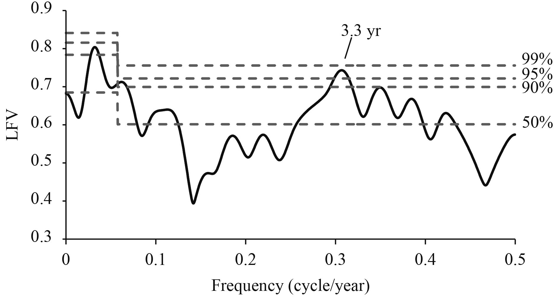
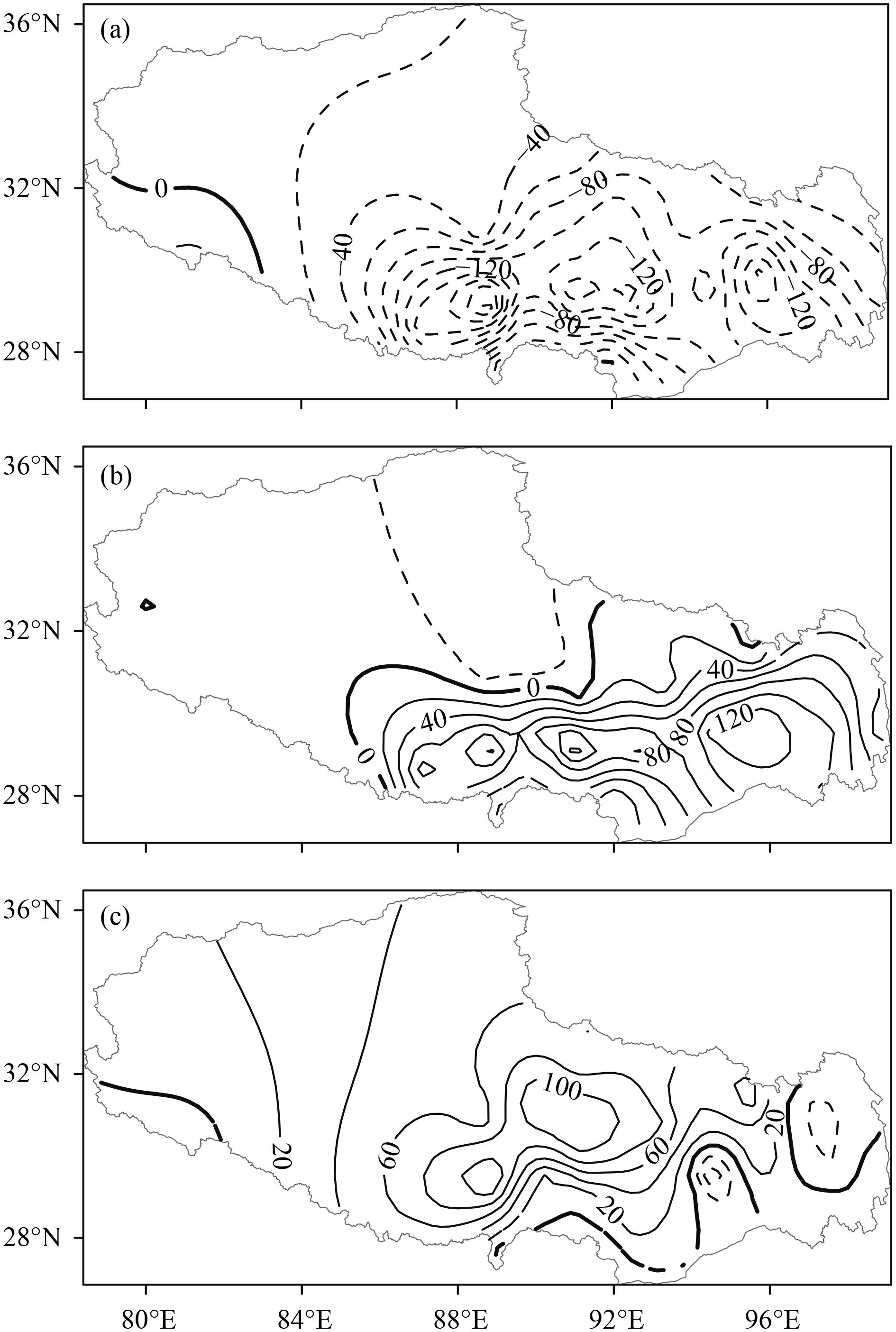
3 Periodic characteristics of precipitationThe MTM-SVD is performed on the RSPT data and the LFV spectrum is shown in Fig. 1. A significant peak (95% confidence level) is seen at 3.3 yr (0.3062 cycles per year (cpy)) on the interannual timescales. The peaks on the inter-decadal timescales do not reach the 50% confidence level. Figure 2 shows the complete cycle of the quasi-3-yr oscillation at phases 0°, 120°, and 240° (with an increment of 1 yr between snap shots). In year 1 (phase 0°), strong negative rainfall anomalies are seen over most of Tibet, in particular a low abnormal center near Shigatse and Lhasa (Fig. 2a). In year 2 (phase 120°), positive rainfall anomalies appear over southeastern Tibet and a high anomaly zone is located downstream of the Yarlung Zangbo River near Shigatse, Linzhi, and Mangkam (Fig. 2b). By year 3 (phase 240°), most of Tibet is dominated by positive rainfall anomalies, except for a few stations in the southeast (Fig. 2c). The location of the anomalies in year 4 return to those of the first year, the start of the next cycle.
|
| Figure 1 LFV spectrum from the MTM-SVD analysis of the RSPT (1981–2015). The dashed lines are the confidence levels of the Monte Carlo simulations. |
|
| Figure 2 Spatial patterns of the reconstructed RSPT (mm) at three consecutive phases of a 3-yr (0.3062 cpy) oscillation. Phases (a) 0°, (b) 120°, and (c) 240° . |
This analysis shows that the RSPT has a significant quasi-3-yr cycle; previous research (Mann and Park, 1996; Apipattanavis et al., 2009) indicated that the ENSO has the characteristics of a 3–7-yr cycle. We therefore investigated whether there is a relationship between these two phenomena. LFV spectral analysis of the combined data field with the RSPT and SST found that the coupling field also has a significant peak in a quasi-3-yr cycle (data omitted).
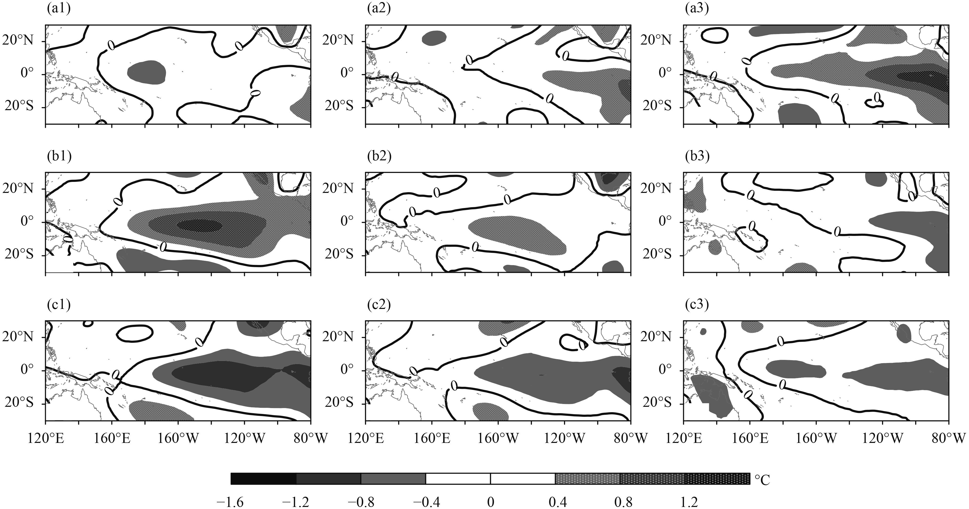
We performed a joint MTM-SVD analysis on the coupling field between the RSPT and the SST (winter, spring, and summer) to identify the variability in the quasi-3-yr cycle in which the two fields exhibit significant coherence. Figure 3 clearly shows that the SST positive anomaly in eastern Pacific in the first year (phase 0°) is first seen in winter and then expands westward in spring until an EP El Niño event is seen in the summer. In the second year (phase 120°), a CP El Niño event is seen in winter, then the SST over the central Pacific decreases, and negative anomalies appear in the east until the summer, when the CP El Niño event completely disappears and is replaced by an EP La Niña event. In the third year (phase 240°), a CP La Niña event appears in the preceding winter, and the SST then increases gradually to the normal range in the summer.
Compared with the quasi-3-yr cycle of the RSPT (Fig. 2), different types of ENSO event correspond to abnormal distributions of the RSPT. When there is an enhanced EP El Niño event, a negative rainfall anomaly appears over the whole of Tibet. However, when the CP El Niño event changes to an EP La Niña event from winter to summer, there is more precipitation in southeastern Tibet and the gradual weakening of the CP La Niña event corresponds to more rainfall over most of Tibet.
|
| Figure 3 Spatial patterns of the reconstructed SST (a1–c1, winter; a2–c2, spring; a3–c3, summer) and RSPT anomalies (in mm) at three consecutive phases of a 3-yr (0.3062 cpy) period oscillation. Phases (a) 0°, (b) 120°, and (c) 240°. |
Another joint analysis was performed between six variables: omega, the vertical shear of the zonal wind, the water vapor transport flux, the 100-hPa height field (Hgt100), the 500-hPa height field (Hgt500), and the RSPT in an attempt to understand the mechanism of the quasi-3-yr oscillation between the ENSO and RSPT. The ENSO event is accompanied by a wide range of SST anomalies in the Pacific Ocean, which lead to changes in the atmospheric circulation affecting the RSPT.
5.1 Responses of the Walker circulationFigure 4 shows the reconstructed spatial patterns of the quasi-3-yr cycle of omega (10°S–10°N) and the RSPT. In phase 0° (Fig. 4a), there are strong negative vertical wind anomalies west of the dateline and a positive anomaly to the east—that is, the Walker circulation is suppressed. In 120° phase (Fig. 4b), the anomalous distribution is the opposite of that in phase 0° and unusual ascending motion is located near 100°E, which enhances the Walker circulation and the main convection area moves westward. In phase 240° (Fig. 4c), the weak positive anomalies in the vertical wind appear near the dateline and 100°W, but negative anomalies are seen near 100°E, which make the Walker circulation similar to the climatological mean (Fig. 4d). Different ENSO events may lead to different distributions of anomalous SST, which change the Walker circulation.

|
| Figure 4 Longitude–height distributions of the reconstructed omega (10° S–10° N) in summer and RSPT anomalies at three consecutive phases of a 3-yr (0.3062 cpy) period oscillation. Phases (a) 0°, (b) 120°, and (c) 240°. (d) is the climatological mean field (10-3 Pa s–1). |
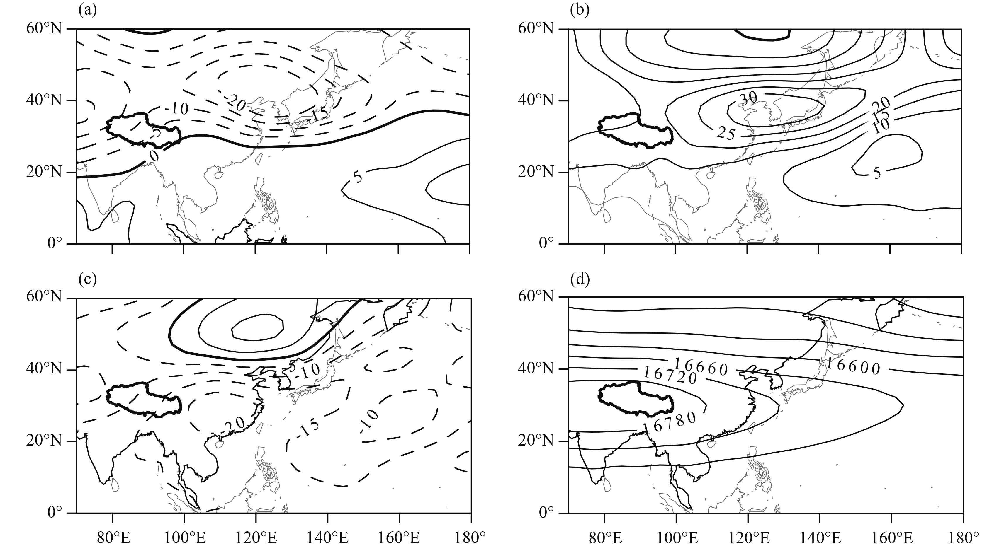
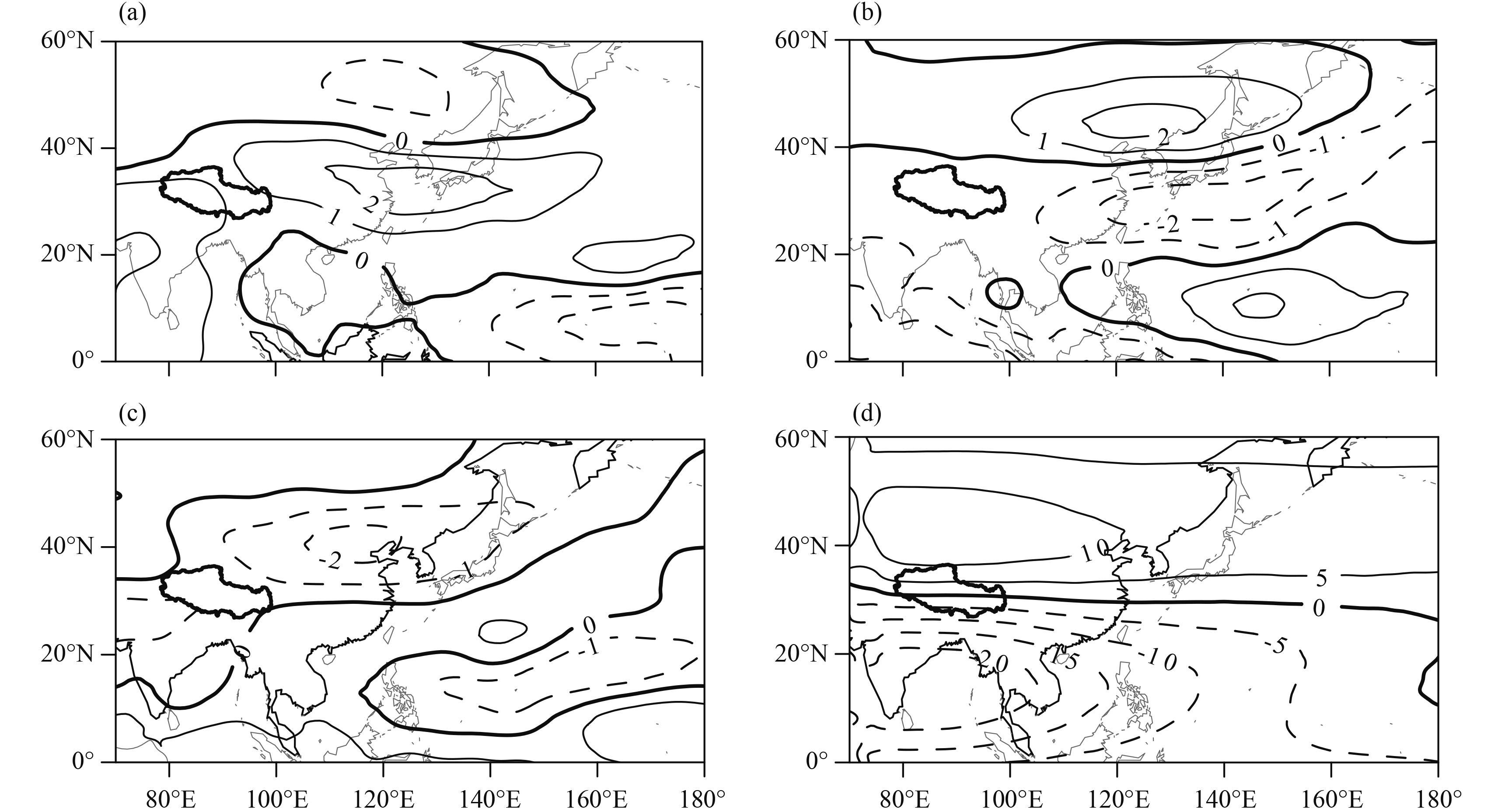
Previous studies have shown that the South Asian high (SAH) is an important component of both Asian summer monsoon systems and that its intensity and location are closely related to the Asian summer monsoon rainfall (Krishnamurti and Bhalme, 1976; Zhang et al., 2002; Wei et al., 2015). Using the same method as before, we reconstructed the quasi-3-yr period of the 100-hPa height field and the RSPT. In phase 0° (Fig. 5a), negative height anomalies are seen in the middle and high latitudes and a positive height anomaly in low latitude regions. The SAH moves southward due to the weak upper easterly wind over the Arabian Sea (Fig. 6a) in the weak Walker circulation pattern. In phase 120° (Fig. 5b), positive height anomalies are seen from low to high latitudes and an abnormal center is seen near 40°N. The SAH moves northward due to the strong upper easterly wind over the Arabian Sea (Fig. 6b) in the strong Walker circulation pattern. In phase 240° (Fig. 5c), a negative height anomaly appears from low to high latitudes. The SAH is weak and moves westward due to both the weak tropical easterly wind and the subtropical westerly wind (Fig. 6c).
|
| Figure 5 Spatial patterns of the reconstructed 100-hPa height field in summer and RSPT anomalies at three consecutive phases of a 3-yr (0.3062 cpy) period oscillation. Phases (a) 0°, (b) 120°, and (c) 240°. (d) is the climatological mean (gpm). |
|
| Figure 6 As in Fig. 5, but for the 100-hPa zonal wind in summer and (d) the climatological mean (m s–1). |
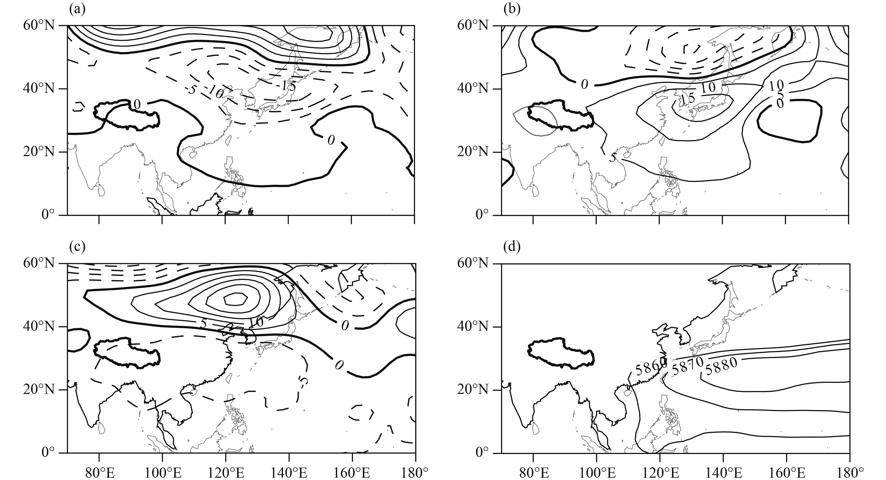
The western Pacific subtropical high (WPSH) is closely associated with the spatiotemporal distribution of summer rainfall in East Asia (Tao and Chen, 1987; Ding, 1994) and has different sensitivities to the two different types of ENSO event (Zang and Wang, 1984; Paek et al., 2015). We reconstructed the quasi-3-yr period of the 500-hPa height field and the RSPT. In phase 0° (Fig. 7a), negative height anomalies appear near 40°N and the WPSH retreats southward. In phase 120° (Fig. 7b), positive height anomalies are seen near Kuroshio, extending the WPSH northwestward and making it stronger. In phase 240° (Fig. 7c), the WPSH is weak and a positive anomaly center appears near northeastern Asia, indicating a more active blocking high. Lu and Huang (1998) also reported that the SST anomalies in the tropical western Pacific are one of the important causes of the inter-annual variation in blocking highs over northeastern Asia.
|
| Figure 7 As in Fig. 5, but for the 500-hPa height field (gpm) in summer. |
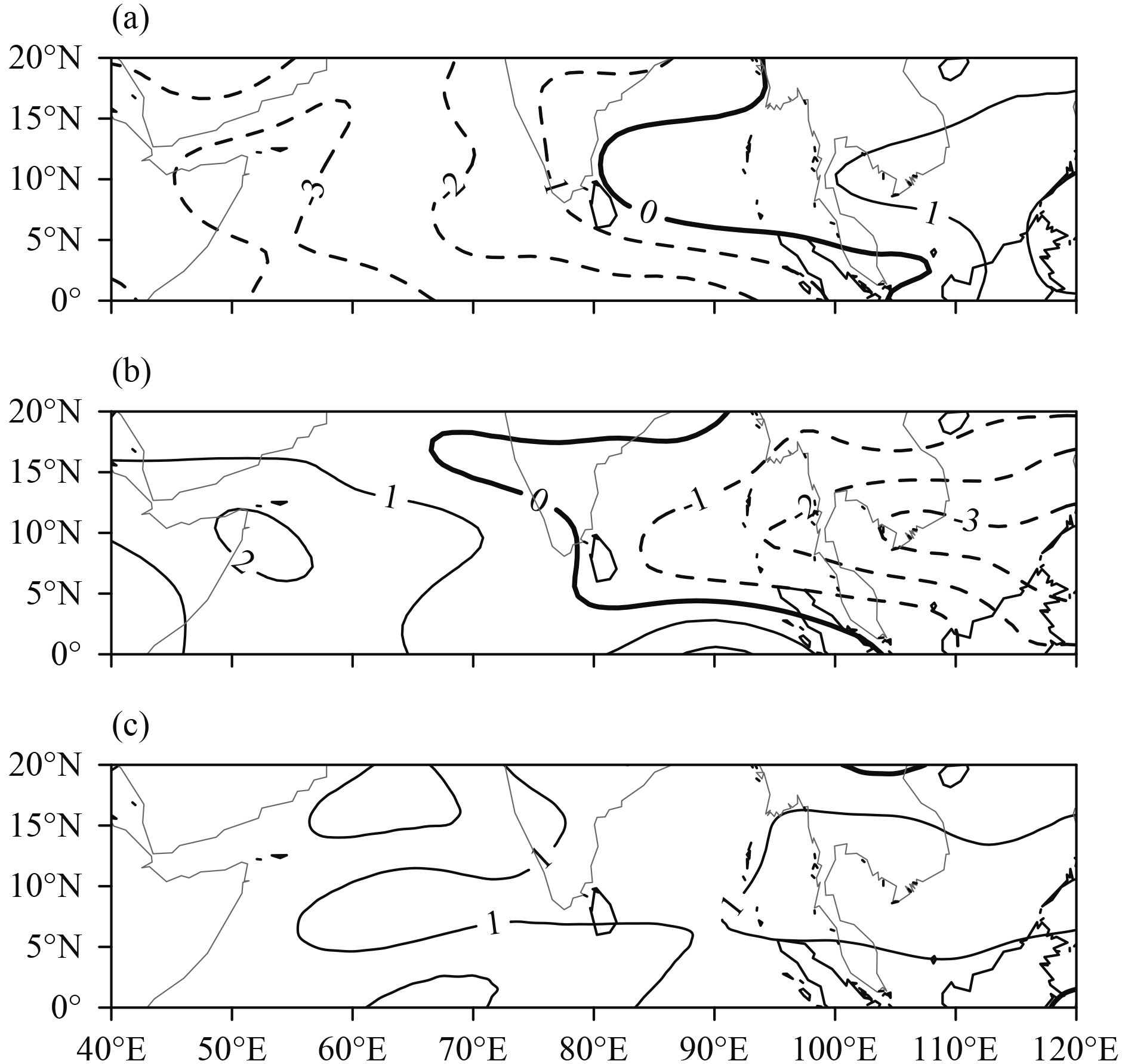
The vertical shear of the zonal wind over the Arabian Sea between 850 and 200 hPa can reflect the intensity of the SASM, which directly affects the amount of precipitation in Southwest China (Webster and Yang, 1992). The 850-hPa zonal wind over the low latitudes of the western North Pacific can affect the western North Pacific summer monsoon (WNPSM), which is an important source of rainfall in China (Wang and Fan, 1999). Figure 8 shows the reconstructed spatial patterns of the vertical shear of zonal wind from northern India Ocean to western North Pacific and the RSPT in the quasi-3-yr cycle, showing both the anomalous SASM and WNPSM. In phase 0° (Fig. 8a), obvious negative anomalies appear west of 90°E over the Arabian Sea, indicating that the SASM is weak. In phase 120° (Fig. 8b), the Arabian Sea shows a significant positive anomaly, whereas the Bay of Bengal and areas to the east show an obvious negative anomaly, suggesting that the SASM is strong and the WNPSM is weak. In phase 240° (Fig. 8c), a significant positive anomaly near the South China Sea indicates that the WNPSM is strong, a similar result to that obtained by Wang et al. (2001)—namely, the WNPSM is negatively correlated with the Niño-3.4 SST anomaly in the preceding winter.
|
| Figure 8 Spatial patterns of the reconstructed vertical shear of the zonal wind (850 minus 200 hPa; m s–1) field in summer and RSPT anomalies at three consecutive phases of a 3-yr (0.3062 cpy) period oscillation. Phases (a) 0°, (b) 120°, and (c) 240°. |
The water vapor flux over China is dominated by the Asian monsoon system (Murakami and Matsumoto, 1994; Li and Zhou, 2012), which directly influences the rainfall (Benton et al., 1950; Simmonds et al., 1999). Figure 9 shows the reconstructed spatial patterns of the water vapor transport flux, divergence, and the RSPT in the quasi-3-yr cycle. In phase 0° (Fig. 9a), easterly anomalies in the water vapor transport fluxes are seen in the Arabian Sea, westerly anomalies from south of the Indochina Peninsula to the Philippines, and a strong divergence in the water vapor flux over Tibet. In phase 120° (Fig. 9b), the distribution of anomalies is in contrast to those in phase 0°. The westerly anomalies in the water vapor transport flux from the Arabian Sea and the easterly anomalies from the Bay of Bengal converge in the Indian Peninsula, bringing an anomalous belt of water vapor to Tibet and a strong convergence of water vapor over southeastern Tibet. In phase 240° (Fig. 9c), cyclonic transport of water vapor is seen in Northwest Pacific, resulting in an easterly transport anomaly from the Sea of Japan to Tibet, causing the convergence of water vapor over Tibet. The relationships between the anomalous distribution of water vapor transport and the ENSO events (Fig. 2) in the relevant phase are similar to those reported by Li et al. (2014).

|
| Figure 9 As in Fig. 8, but for the water vapor transport flux field (vectors; kg m–1 s–1) and the divergence field (shaded; 10–5 kg m–2 s–1) from 1000 to 300 hPa in summer. |
Using MTM-SVD analysis, we identified a quasi-3-yr cycle in the RSPT with a typical circulation pattern of less–more–more precipitation. The coupling field be-tween the RSPT and the SSTs in the Pacific Ocean also has a significant quasi-3-yr cycle, indicating that particular ENSO events can result in particular anomalies of the RSPT in the corresponding phase.
We analyzed the coupling of atmospheric circulation variables with the RSPT using the joint MTM-SVD method and established conceptual models during a typical 3-yr cycle. In the first year, the gradually developing EP El Niño events accompanied by positive SST anomalies in East Pacific restrain the Walker circulation. This weakens the SASM and reduces the transport of water vapor from the southwest. The SAH and WPSH both move southward and the overall result is less precipitation in Tibet.
In the second year, the conversion of the CP El Niño events to the EP La Niña events warms the western Pacific warm pool and cools the eastern equatorial Pacific, which strengthens the Walker circulation and extends the ascending area westward. This results in a more active SASM over the Arabian Sea, which brings more water vapor directly to Tibet. The SAH moves eastward and the WPSHs move westward.
In the third year, the CP La Niña events decrease and the SST anomaly over the central Pacific gradually returns from winter to summer. This leads to a strong westward propagation of the SASM, forcing the cyclonic convergence of water vapor in Northwest Pacific. Blocking highs appear over northeastern Asia, causing transport of easterly anomalies from the Sea of Japan to Tibet and increased precipitation in Tibet.
| Apipattanavis, S., G. J. McCabe, B. Rajagopalan, et al., 2009: Joint spatiotemporal variability of global sea surface temperatures and global Palmer drought severity index values. J. Climate, 22, 6251–6267. DOI:10.1175/2009JCLI2791.1 |
| Benton, G. S., R. T. Blackburn, and V. O. Snead, 1950: The role of the atmosphere in the hydrologic cycle. Eos, Trans. Amer. Geophys. Union, 31, 61–73. DOI:10.1029/TR031i001p00061 |
| Ding, Y. H., 1994: The summer monsoon in East Asia. Monsoons over China. Ding, Y. H. Ed., Kluwer Academic, Boston, 1–9, doi: 10.1007/978-94-015-8302-2_1. |
| Du, J., and Y. C. Ma, 2004: Climatic trend of rainfall over Tibetan Plateau from 1971 to 2000. Acta Geographica Sinica, 59, 375–382. DOI:10.11821/xb200403007 |
| Fu, C. B., and J. Fletcher, 1985: Two types of warming at the equator during El Niño. Chin. Sci. Bull., 8, 596–599. DOI:10.1360/csb1985-30-8-596 |
| Han, X., F. Y. Wei, Y. M. Tourre, et al., 2008: Spatio-temporal variability of Northern Hemispheric sea level pressure (SLP) and precipitation over the mid-to-low reaches of the Yangtze River. Adv. Atmos. Sci., 25, 458–466. DOI:10.1007/s00376-008-0458-x |
| Huang, X. Q., C. R. Luobu, Y. Yang, et al., 2013: Temporal and spatial variation of precipitation events frequency and intensity in rainy season during 1961–2007 in Tibet, China. J. Desert Res., 33, 902–910. DOI:10.7522/j.issn.1000-694X.1013.00088 |
| Jin, Z. H., and S. Y. Tao, 1999: A study on the relationships between ENSO cycle and rainfalls during summer and winter in eastern China. Chinese J. Atmos. Sci., 23, 663–672. DOI:10.3878/j.issn.1006-9895.1999.06.03 |
| Krishnamurti, T. N., and H. N. Bhalme, 1976: Oscillations of a monsoon system. Part I: Observational aspects. J. Atmos. Sci., 33, 1937–1954. DOI:10.1175/1520-0469(1976)033 |
| Kug, J. S., F. F. Jin, and S. I. An, 2009: Two types of El Niño events: Cold tongue El Niño and warm pool El Niño. J. Climate, 22, 1499–1515. DOI:10.1175/2008JCLI2624.1 |
| Li, X. Z., and W. Zhou, 2012: Quasi-4-yr coupling between El Niño–Southern Oscillation and water vapor transport over East Asia–WNP. J. Climate, 25, 5879–5891. DOI:10.1175/JCLI-D-11-00433.1 |
| Li, X. Z., W. Zhou, D. L. Chen, et al., 2014: Water vapor transport and moisture budget over eastern China: Remote forcing from the two types of El Niño. J. Climate, 27, 8778–8792. DOI:10.1175/JCLI-D-14-00049.1 |
| Liu, X. D., and Z.-Y. Yin, 2001: Spatial and temporal variation of summer precipitation over the eastern Tibetan Plateau and the North Atlantic oscillation. J. Climate, 14, 2896–2909. DOI:10.1175/1520-0442(2001)014 |
| Lu, H. L., Q. Q. Shao, J. Y. Liu, et al., 2008: Cluster analysis on summer precipitation field over Qinghai–Tibetan Plateau from 1961 to 2004. J. Geogr. Sci., 18, 295–307. DOI:10.1007/s11442-008-0295-y |
| Lu, R. Y., and R. H. Huang, 1998: Influence of East Asia/Pacific teleconnection pattern on the interannual variations of the blocking highs over the northeastern Asia in summer. Scientia Atmospherica Sinica, 22, 727–734. DOI:10.3878/j.issn.1006-9895.1998.05.07 |
| Mann, M. E., and J. Park, 1994: Global-scale modes of surface temperature variability on interannual to century timescales. J. Geophys. Res., 99, 25819–25833. DOI:10.1029/94JD02396 |
| Mann, M. E., and J. Park, 1996: Joint spatiotemporal modes of surface temperature and sea level pressure variability in the Northern Hemisphere during the last century. J. Climate, 9, 2137–2162. DOI:10.1175/1520-0442(1996)009 |
| Mann, M. E., and J. Park, 1999: Oscillatory spatiotemporal signal detection in climate studies: A multiple-taper spectral domain approach. Adv. Geophys., 41, 1–131. DOI:10.1016/S0065-2687(08)60026-6 |
| Minobe, S., 2000: Spatio-temporal structure of the pentadecadal variability over the North Pacific. Prog. Oceanogr., 47, 381–408. DOI:10.1016/S0079-6611(00)00042-2 |
| Murakami, T., and J. Matsumoto, 1994: Summer monsoon over the Asian continent and western North Pacific. J. Meteor. Soc. Japan, 72, 719–745. DOI:10.2151/jmsj1965.72.5_719 |
| Paek, H. J., J. Y. Yu, J. W. Hwu, et al., 2015: A source of AGCM bias in simulating the western Pacific subtropical high: Different sensitivities to the two types of ENSO. Mon. Wea. Rev., 143, 2348–2362. DOI:10.1175/MWR-D-14-00401.1 |
| Pubu, Z. M., S. W. Zhou, and Y. H. Fu, 2002: Reflection from the ENSO event on precipitation during the summer of Tibet. Tibet’s Science & Technology, 2, 41–47. DOI:10.3969/j.issn.1004-3403.2002.02.017 |
| Simmonds, I., D. H. Bi, and P. Hope, 1999: Atmospheric water vapor flux and its association with rainfall over China in summer. J. Climate, 12, 1353–1367. DOI:10.1175/1520-0442(1999)012 |
| Small, D., and S. Islam, 2008: Low frequency variability in fall precipitation across the United States. Water Resour. Res., 44, W04426. DOI:10.1029/2006WR005623 |
| Tao, S.-Y., and Y.-H. Ding, 1981: Observational evidence of the influence of the Qinghai–Xizang (Tibet) Plateau on the occurrence of heavy rain and severe convective storms in China. Bull. Amer. Meteor. Soc., 62, 23–30. DOI:10.1175/1520-0477(1981)062 |
| Tao, S. Y., and L. X. Chen, 1987: A review of recent research on the East Asian summer monsoon in China. Monsoon Meteorology. C. P. Chang and T. N. Krishnamurti, Eds., Oxford University Press, Oxford, pp. 60-92. |
| Wang, B., and Z. Fan, 1999: Choice of South Asian summer monsoon indices. Bull. Amer. Meteor. Soc., 80, 629–638. DOI:10.1175/1520-0477(1999)080 |
| Wang, B., R. Wu, and K.-M. Lau, 2001: Interannual variability of Asian summer monsoon: Contrast between the Indian and western North Pacific–East Asian monsoons. J. Climate, 14, 4073–4090. DOI:https://doi.org/10.1175/1520-0442(2001)014,4073:IVOTAS.2.0.CO;2 |
| Webster, P. J., and S. Yang, 1992: Monsoon and ENSO: Selectively interactive systems. Quart. J. Roy. Meteor. Soc., 118, 877–926. DOI:10.1002/qj.49711850705 |
| Wei, W., R. H. Zhang, M. Wen, et al., 2015: Interannual variation of the South Asian high and its relation with Indian and East Asian summer monsoon rainfall. J. Climate, 28, 2623–2634. DOI:10.1175/JCLI-D-14-00454.1 |
| Wu, G. X., and Y. M. Liu, 2016: Impacts of the Tibetan Plateau on Asian climate. Meteor. Monogr., 56, 7.1–7.29. DOI:10.1175/AMSMONOGRAPHS-D-15-0018.1 |
| Yanai, M., C. F. Li, and Z. S. Song, 1992: Seasonal heating of the Tibetan Plateau and its effects on the evolution of the Asian summer monsoon. J. Meteor. Soc. Japan, 70, 319–351. DOI:10.2151/jmsj1965.70.1B_319 |
| Ye, D. Z., 1981: Some characteristics of the summer circulation over the Qinghai–Xizang (Tibet) Plateau and its neighborhood. Bull. Amer. Meteor. Soc., 62, 14–19. DOI:10.1175/1520-0477(1981)062 |
| Yeh, S. W., J. S. Kug, B. Dewitte, et al., 2009: El Niño in a changing climate. Nature, 461, 511–514. DOI:10.1038/nature08316 |
| Yuan, Y., and S. Yang, 2012: Impacts of different types of El Niño on the East Asian climate: Focus on ENSO cycles. J. Climate, 25, 7702–7722. DOI:10.1175/JCLI-D-11-00576.1 |
| Zang, H. F., and S. W. Wang, 1984: Equatorial eastern Pacific SST and subtropical high. Acta Oceanol. Sinica, 3, 471–476. |
| Zhang, Q., G. X. Wu, and Y. F. Qian, 2002: The bimodality of the 100-hPa South Asian high and its relationship to the climate anomaly over East Asia in summer. J. Meteor. Soc. Japan, 80, 733–744. DOI:10.2151/jmsj.80.733 |
| Zheng, Q. L., and K.-N. Liou, 1986: Dynamic and thermodynamic influences of the Tibetan Plateau on the atmosphere in a general circulation model. J. Atmos. Sci., 43, 1340–1355. DOI:10.1175/1520-0469(1986)043 |
| Zhou, S. W., Z. M. Pubu, and L. Jia, 2000: Analysis of rainfall patterns during rainy season over the Tibetan Plateau. Meteor. Mon., 26, 39–43. DOI:10.3969/j.issn.1000-0526.2000.05.010 |
 2018, Vol. 32


