The Chinese Meteorological Society
Article Information
- YAN, Bing, Sixun HUANG, and Jing FENG, 2017.
- Retrieval of Eddy Thermal Conductivity in the Weakly Nonlinear Prandtl Model for Katabatic Flows. 2017.
- J. Meteor. Res., 31(5): 965-975
- http://dx.doi.org/10.1007/s13351-017-7025-2
Article History
- Received February 19, 2017
- in final form July 3, 2017
2. State Key Laboratory of Satellite Ocean Environment Dynamics, Second Institute of Oceanography, State Oceanic Administration, Hangzhou 310012

Planetary atmospheric boundary layer research has long been a popular field in atmospheric sciences (Mahrt, 1982, 1998; Tan et al., 2006; Baklanov et al., 2011). Studies have shown that anabatic and katabatic flows occurring in the boundary layer affect glacial mass variation, sea level rise, and climate change; thus, these processes are under the scientific spotlight (Grisogono and Oerlemans, 2001a; Barthélemy et al., 2012; Grisogono et al., 2015; Salvador et al., 2016). Katabatic and anabatic winds occur over a sloped surface. When the temperature of an air parcel near a sloping surface falls, a difference between it and the ambient temperature at the same elevation is established. The buoyancy force related to this temperature contrast projects in the along-slope direction and induces the katabatic wind. Its counterpart, i.e., anabatic wind, corresponds to heating over a sloping surface (Shapiro et al., 2012). Research on the modeling and theory of a stably stratified atmospheric boundary layer is an active field (Grisogono and Oerlemans, 2001b; Grisogono, 2003; Baklanov et al., 2011; Ingel, 2011; Grisogono et al., 2015). Flows over sloping terrain have been simulated with numerical weather prediction and climate models (Smith and Skyllingstad, 2005; Jeričević et al., 2010; De Ridder et al., 2015). However, the handling of the relevant lower boundary conditions and near-surface turbulence parameterization remains unresolved (Epifanio, 2007; Buzzi et al., 2011). Therefore, researchers continue to focus their attention on anabatic and katabatic flows (Shapiro et al., 2012).
Among the studies on anabatic and katabatic flows, simulation based on analytical modeling is the most fundamental. Most analytical models of katabatic flows are one dimensional; furthermore, the most common analytical model of thermally driven simple slope flows is the Prandtl model (Egger, 1990; Axelsen and van Dop, 2009). The strengths and weaknesses of the classical Prandtl model have been explored by Grisogono and Axelsen (2012), mainly in large eddy simulations based on limited observational data (van den Broeke, 1997). This line of work was improved by Mo (2013); however, serious limitations remain, not least insofar as most analytical models of katabatic flow are linear and the eddy thermal conductivity is assumed to be constant. The main disadvantage of a linear Prandtl model is that the thermodynamic equation does not consider the fact that the flow-related potential temperature gradient near the surface feeds back to the environmental potential temperature gradient (Grisogono et al., 2015).
The abovementioned defect of the classical Prandtl model was improved by Grisogono et al. (2015), who introduced a small parameter ε into the thermodynamic equilibrium equation that controls the transport from the flow-induced potential temperature gradient to the environment. The addition of this parameter makes the model more realistic, as it transforms from a linear model into a weakly nonlinear model. The scope of the small parame-ter
A second disadvantage of the classical Prandtl model was amended by assuming gradually varying eddy thermal conductivity K; that is, K is a function of height z (Grisogono and Oerlemans, 2001a,b, 2002), which is closer to reality. Shapiro et al. (2016) found that the time-varying eddy thermal conductivity K was potentially more significant than the vertical change when they studied the Great Plains nocturnal low-level jet. Because our research is based on the weakly nonlinear Prandtl model in the stable boundary layer, the vertical change in K is our main concern. However, the varying K(z) is generally obtained by an empirical parameterization scheme, which is an approximation of reality. Thus, it is worth studying how to precisely retrieve the varying eddy thermal conductivity.
As is well known, the problems in parameter retrieval are difficult to resolve because they are generally nonlinear and sometimes ill-posed. Indeed, there are still many important theoretical issues being investigated (Huang et al., 2006). Parameter retrieval via inversion is an approach that has been successfully applied in many disciplines, such as the geosciences, biological sciences, and atmospheric and oceanic sciences. Some previous studies on inverse problems can be found in Huang et al. (2005), Zhao and Huang (2012), and Yan and Huang (2014). Typically, parameter inversion is mainly tackled by using the variational method and Kalman filter me-thod, and there have been many studies conducted using boundary layer parameter inversion. For example, Hu et al. (2010) explored the treatment of model errors and uncertainties through simultaneous state and parameter estimation with an ensemble Kalman filter (EnKF). Nielsen-Gammon et al. (2010) evaluated the sensitivities of a planetary boundary layer scheme for parameter estimation with an EnKF. Huang et al. (2005) analyzed the retrieval of atmospheric and oceanic parameters with variational data assimilation and the relevant numerical calculation. Zhao and Huang (2012) retrieved atmos-pheric refractivity profiles from sea surface backscattered radar clutter with a variational method.
As for the retrieval of gradually varying K(z), this too is a typical parameter retrieval problem. In both the atmospheric sciences and the hydromechanics research, K(z) is a critical parameter and is usually derived from an empirical parameterization scheme. It is actually very difficult to obtain K because it is closely related to the dynamic thermal structure of the fluid. It would therefore be an important step to develop a method that can achieve a reasonable retrieval of K(z) in the weakly nonlinear Prandtl model, as this would be highly useful in improving theoretical analyses and numerical models.
This paper describes the retrieval of eddy thermal conductivity in the weakly nonlinear Prandtl model through the variational assimilation method. Because observational data are difficult to obtain, we demonstrate the effectiveness and reliability of the method through numerical experiments.
The rest of this paper is arranged as follows. Section 2 introduces the weakly nonlinear Prandtl model; Section 3 describes the variational assimilation scheme for the model; Section 4 reports the numerical experiment results; and finally, Section 5 provides a summary and discussion. Details of the Wentzel–Kramers–Brillouin (WKB) calculation steps are also included, in the Appendix.
2 Weakly nonlinear Prandtl model 2.1 ModelThe classical Prandtl model has been validated and used by numerous scientists and engineers over the past few decades (Mahrt, 1982; Egger, 1990; Axelsen and van Dop, 2009). This linear model is imperfect, given that the actual physical process is generally nonlinear. In the past decade, the model has been modified to more accurately represent the real physical process. Among these improvements, introducing the small parameter
The weakly nonlinear Prandtl model is essentially a simplified, steady-state, one-dimensional model with governing equations in the tilted coordinate system and with a constant slope α,
| $\begin{split}& g\frac{\theta }{{{\Theta _{\rm{0}}}}}\sin (\alpha) + K\Pr \frac{{{\partial ^2}u}}{{\partial {z^2}}} = 0, \\ & - (\Gamma + \varepsilon \frac{{\partial \theta }}{{\partial z}})u\sin (\alpha) + K\frac{{{\partial ^2}\theta }}{{\partial {z^2}}} = 0.\end{split}$ | (1) |
The term
|
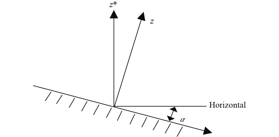
| Figure 1 Slope coordinate system. The downslope is inclined at an angle (α) to the horizontal; z is the coordinate that is perpendicular to the slope surface; z* represents the true vertical direction, which is perpendicular to the horizontal. |
The forward problem of the weakly nonlinear Prandtl model is a weakly nonlinear two-point boundary value problem. Because of
| $\begin{array}{l}u = {u_0} + \varepsilon {u_1} + \varepsilon u_2^2 + \cdot \cdot \cdot, \\\theta = {\theta _0} + \varepsilon {\theta _1} + \varepsilon \theta _2^2 + \cdot \cdot \cdot, \end{array}$ | (2) |
where the subscripts represent the order of expansion, with zero-order flow variables being the solution for the classic Prandtl model, and the addition to first-order corrections being the solution for the weakly nonlinear mo-del. We maintain this expansion only for the first-order corrections. By substituting Eq. (2) into Eq. (1), the solution for the zero-order expansion is obtained, i.e., the solution for the classical Prandtl model (Mahrt, 1998; Grisogono and Oerlemans, 2002; Stiperski et al., 2007) is
| $\frac{{{{\rm d}^4}({u_0}, {\theta _0})}}{{{\rm d}{z^4}}} + {N^2}\frac{{{{\sin }^2}(\alpha)}}{{\Pr K\!{{(z)}^2}}}({u_0}, {\theta _0}) = 0, $ | (3) |
where
| $\begin{array}{l}{u_0} = - C\mu \exp [ - I]\sin [I], \\{\theta _0} = C\exp [ - I]\cos [I], \end{array}$ | (4) |
where C is the surface potential temperature deficit in the case of katabatic flows;
The solution for the first-order corrections
| $\begin{split}& g\frac{{{\theta _1}}}{{{\Theta _0}}}\sin (\alpha) + K\Pr \frac{{{{\rm d}^2}{u_1}}}{{{\rm d}{z^2}}} = 0, \\& - (\Gamma {u_1} + \frac{{{\rm d}{\theta _0}}}{{{\rm d}z}}{u_0})\sin (\alpha) + K\frac{{{{\rm d}^2}{\theta _1}}}{{{\rm d}{z^2}}} = 0.\end{split}$ | (5) |
Similarly, as before, Eq. (5) can be transformed into:
| $\begin{array}{c} \frac{{{{\rm d}^4}{u_1}}}{{{\rm d}{z^4}}} + {N^2}\frac{{{{\sin }^2}(\alpha)}}{{\Pr K\!{{(z)}^2}}}{u_1} = - \frac{{g{{\sin }^2}(\alpha)}}{{{\Theta _0}K\!{{(z)}^2}\Pr }}{u_0}\frac{{{\rm d}{\theta _0}}}{{{\rm d}z}}, \\\!\!\!\!\! \frac{{{{\rm d}^4}{\theta _1}}}{{{\rm d}{z^4}}} + {N^2}\frac{{{{\sin }^2}(\alpha)}}{{\Pr K\!{{(z)}^2}}}{\theta _1} = \frac{{\sin (\alpha)}}{{K\!(z)}}\frac{{{{\rm d}^2}}}{{{\rm d}{z^2}}}({u_0}\frac{{{\rm d}{\theta _0}}}{{{\rm d}z}}).\end{array}$ | (6) |
The associated boundary conditions are:
For details of the calculation steps, please refer to the Appendix. The form of the solution is obtained as follows:
| $\begin{aligned}{u_1} & = {u_A}\exp (- I)[ - \frac{1}{3}\sin (I) + \frac{2}{{15}}\cos (I)] \\ & + {u_A}\exp (- 2I)[\frac{1}{{30}}\sin (2I) - \frac{1}{{30}}\cos (2I) - \frac{1}{{10}}], \\{\theta _1} & = {\theta _A}\exp (- I)[ - \frac{1}{{15}}\sin (I) - \frac{1}{6}\cos (I)] \\ &+ {\theta _A}\exp (- 2I)[\frac{1}{{15}}\sin (2I) + \frac{1}{{15}}\cos (2I) + \frac{1}{{10}}], \end{aligned}$ | (7) |
where
Thus, the total WKB approximate solutions, up to the first order, are as follows:
| $\begin{array}{l}u = {u_0} + \varepsilon {u_1}, \\\theta = {\theta _0} + \varepsilon {\theta _1}.\end{array}$ | (8) |
The idea of variational data assimilation was proposed by the atmospheric science community in the 1980s (Lorenc, 1988; Gao et al., 1995; Navon, 1998). The primary idea of variational assimilation technology is to combine the model and observation data to obtain the optimal model parameter or model initial value. The essence of this method is optimal control theory (Tosaka et al., 1999). After decades of development, variational assimilation has become a very mature method and has been implemented in operational models. Thus, we use the variational assimilation method to retrieve the eddy thermal conductivity in the weakly nonlinear Prandtl model for katabatic flows.
3.1 Defining the cost functionLet
| $J[{K_0}, h] \!=\! \frac{1}{2}\int_0^H \!\! {[{{(u \!-\! {u^{{\rm {obs}}}})}^2} \!+\! \gamma {{(\theta \!-\! {\theta ^{\rm {obs}}})}^2}]{\rm d}z} {\rm{ = }}\min, $ | (9) |
where
According to the form of variation:
| $\begin{aligned}\delta J & = \int_0^H {[(u - {u^{{\rm {obs}}}})\delta u + \gamma (\theta - {\theta ^{{\rm {obs}}}})\delta \theta ]} {{\rm d}z}\\ & = \int_0^H {[(u - {u^{{\rm {obs}}}})(\frac{{\partial u}}{{\partial I}}\delta I + \frac{{\partial u}}{{\partial K}}\delta K) + \gamma (\theta - {\theta ^{{\rm {obs}}}})(\frac{{\partial \theta }}{{\partial I}}\delta I + \frac{{\partial \theta }}{{\partial K}}\delta K)]} {{\rm d}z}\\ & = \int_0^H {(u - {u^{{\rm {obs}}}})[\frac{{\partial u}}{{\partial I}}(\frac{{\partial I}}{{\partial K}}, \delta K) + \frac{{\partial u}}{{\partial K}}\delta K]{{\rm d}z}} \\ &{\rm{ + }}\int_0^H {\gamma (\theta - {\theta ^{{\rm {obs}}}})[\frac{{\partial \theta }}{{\partial I}}(\frac{{\partial I}}{{\partial K}}, \delta K) + \frac{{\partial \theta }}{{\partial K}}\delta K]{{\rm d}z}} \\ & = \int_0^H {(u - {u^{{\rm {obs}}}})[\frac{{\partial u}}{{\partial I}}(\frac{{\partial I}}{{\partial K}}, \frac{{\partial K}}{{\partial {K_0}}}\delta {K_0} + \frac{{\partial K}}{{\partial h}}\delta h) + \frac{{\partial u}}{{\partial K}}(\frac{{\partial K}}{{\partial {K_0}}}\delta {K_0} + \frac{{\partial K}}{{\partial h}}\delta h)]{{\rm d}z}} \\ & + \int_0^H {\gamma (\theta - {\theta ^{{\rm {obs}}}})[\frac{{\partial \theta }}{{\partial I}}(\frac{{\partial I}}{{\partial K}}, \frac{{\partial K}}{{\partial {K_0}}}\delta {K_0} + \frac{{\partial K}}{{\partial h}}\delta h) + \frac{{\partial \theta }}{{\partial K}}(\frac{{\partial K}}{{\partial {K_0}}}\delta {K_0} + \frac{{\partial K}}{{\partial h}}\delta h)]} {{\rm d}z}.\end{aligned}$ | (10) |
Here,
| $\begin{array}{l}{\nabla _{{K_0}}}J = \int_0^H [{(u - {u^{{\rm {obs}}}})(\frac{{\partial u}}{{\partial I}}(\frac{{\partial I}}{{\partial K}}, \frac{{\partial K}}{{\partial {K_0}}}) + \frac{{\partial u}}{{\partial K}}\frac{{\partial K}}{{\partial {K_0}}}) + \gamma (\theta - {\theta ^{{\rm {obs}}}})(\frac{{\partial \theta }}{{\partial I}}(\frac{{\partial I}}{{\partial K}}, \frac{{\partial K}}{{\partial {K_0}}}) + \frac{{\partial \theta }}{{\partial K}}\frac{{\partial K}}{{\partial {K_0}}})]{{\rm {d}}z}}, \\{\nabla _h}J = \int_0^H [{(u - {u^{{\rm {obs}}}})(\frac{{\partial u}}{{\partial I}}(\frac{{\partial I}}{{\partial K}}, \frac{{\partial K}}{{\partial h}}) + \frac{{\partial u}}{{\partial K}}\frac{{\partial K}}{{\partial h}}) + \gamma (\theta - {\theta ^{{\rm {obs}}}})(\frac{{\partial \theta }}{{\partial I}}(\frac{{\partial I}}{{\partial K}}, \frac{{\partial K}}{{\partial h}}) + \frac{{\partial \theta }}{{\partial K}}\frac{{\partial K}}{{\partial h}})]{{\rm {d}}z}} .\end{array}$ | (11) |
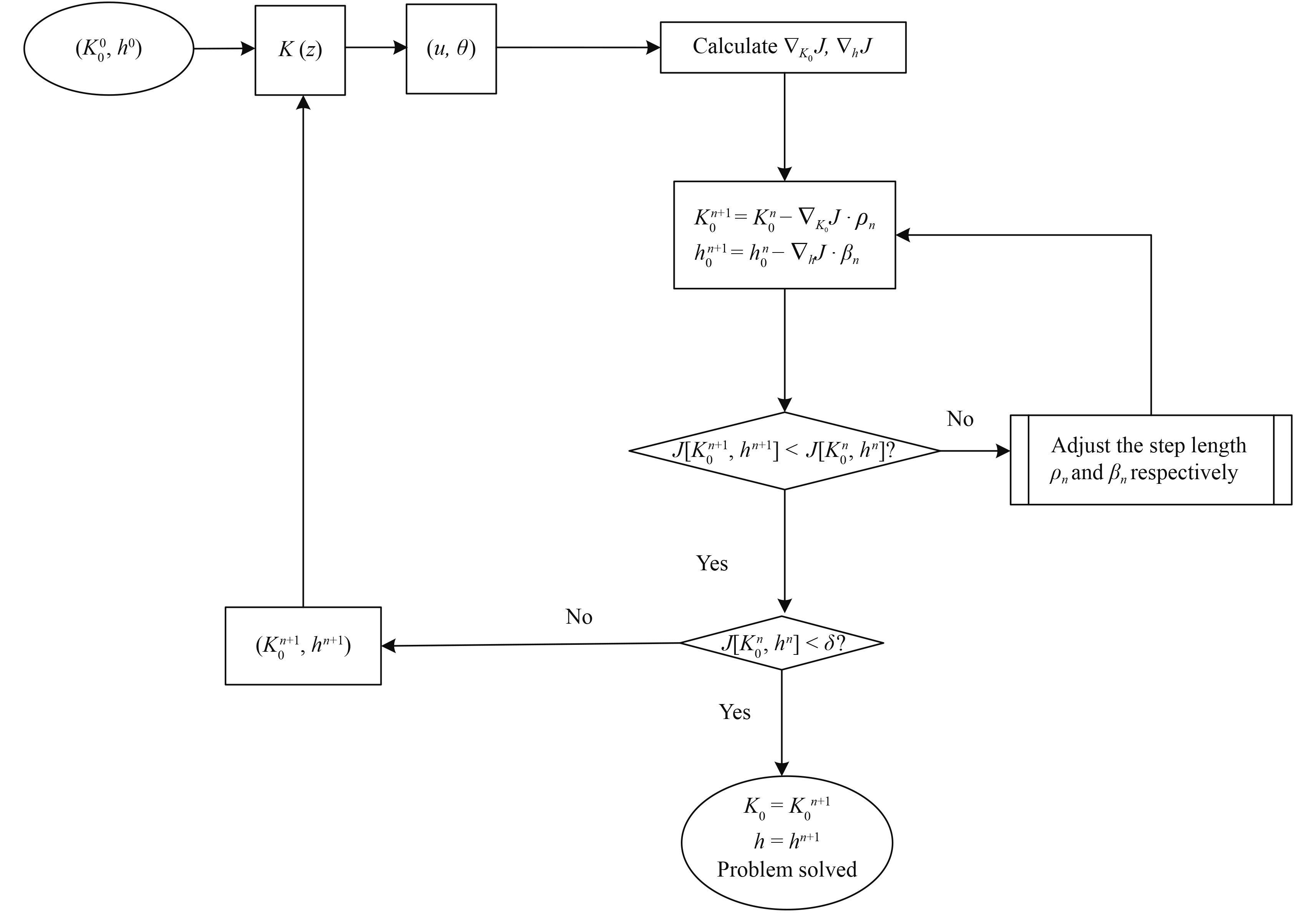
In this paper, the steepest descent method is selected for numerical calculation. The procedure is as follows:
Step 1: Prescribe an initial value for
Step 2: Calculate K(z) according to the formula
Step 3: obtain the solution for the weakly nonlinear Prandtl model through the WKB method and the known parameter;
Step 4: Compute the gradient
Step 5: Set a step length, find the value of
Step 6: Print the result if the cost function is smaller than a very small value; otherwise, replace
A flow chart illustrating the numerical calculation is provided in Fig. 2.
|
| Figure 2 Flow chart of the numerical calculation. |
The initial value is ideally supposed to be logical. It should not be too far away from the truth. We take
To validate the robustness and reliability of the proposed method for parameter retrieval in the weakly nonlinear Prandtl model of katabatic flows, numerical testing is carried out through two experiments, each with two versions: observation with errors and without errors. Near-surface observation data with high accuracy are difficult to obtain; therefore, in this paper, we only use the numerical experiment with simulated observation data to test the proposed method.
However, when validating the proposed method with simulated observations, a problem emerges insofar as the observations are highly dependent on the model (Arnold and Dey, 1986). Considering the independence of the data to the model, we decide to take
Assuming
|
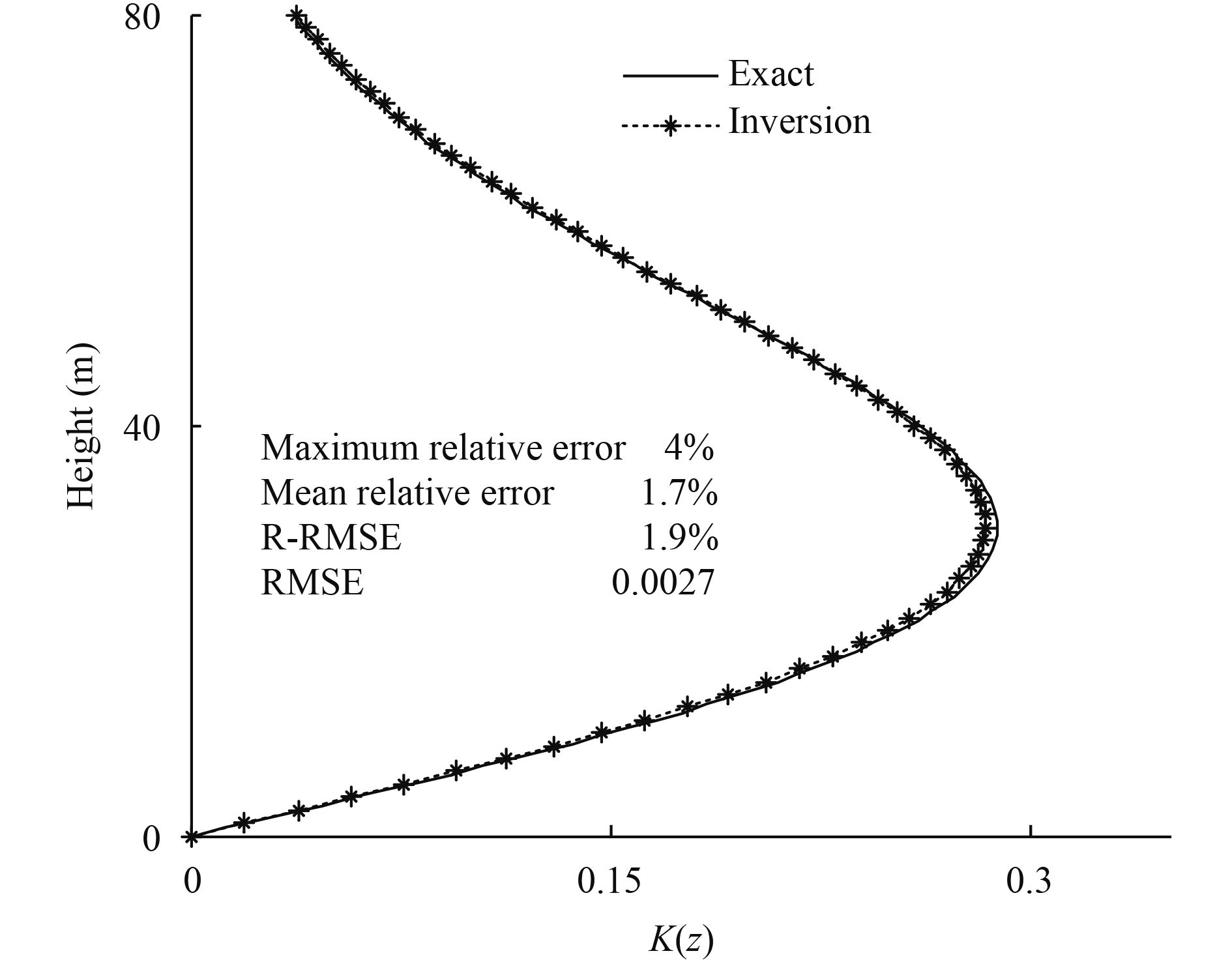
| Figure 3 Comparison between the inversion value of K(z) and the exact value under the condition of observation without noise. The horizontal coordinate represents the value of the eddy thermal conductivity, while the vertical coordinate represents the height. The solid line represents the exact value, and the dashed line with asterisks represents the inversion value of K(z). |
The error mainly arises in the region of maximum K. The maximum absolute error is 0.005, which is small compared with the maximum value of K. The maximum relative error is about 4%, and the mean relative error is about 1.7%. The R-RMSE is 1.9%, and the RMSE is 0.0027. The result demonstrates that the proposed me-thod is effective for observations without noise.
4.1.2 Case Ⅱ:The proposed variational assimilation scheme is robust; it can restrain the influence of the observation error. We illustrate this characteristic in the numerical experiment of Case II. The values of all the parameters are the same as in Case I. Assuming there is random noise with the observation, and the error disturbance has a normal distribution with mean of 0 and standard variance of 0.3. The random noises imposed on wind speed and potential temperature are shown in Fig. 4a, b. The random observation errors depicted by Fig. 4 are expected to represent the real observation errors to the most reasonable degree.

|
| Figure 4 Randomly disturbed (a) wind speed and (b) potential temperature used in the experiment, where the smooth solid line represents the observation without errors and the irregular dashed line with asterisks represents the observation with errors. The noise disturbance is in accordance with the normal distribution (average value is 0; standard variance is 0.3). The observation is discrete, represented by the asterisks along the dashed line. |
|
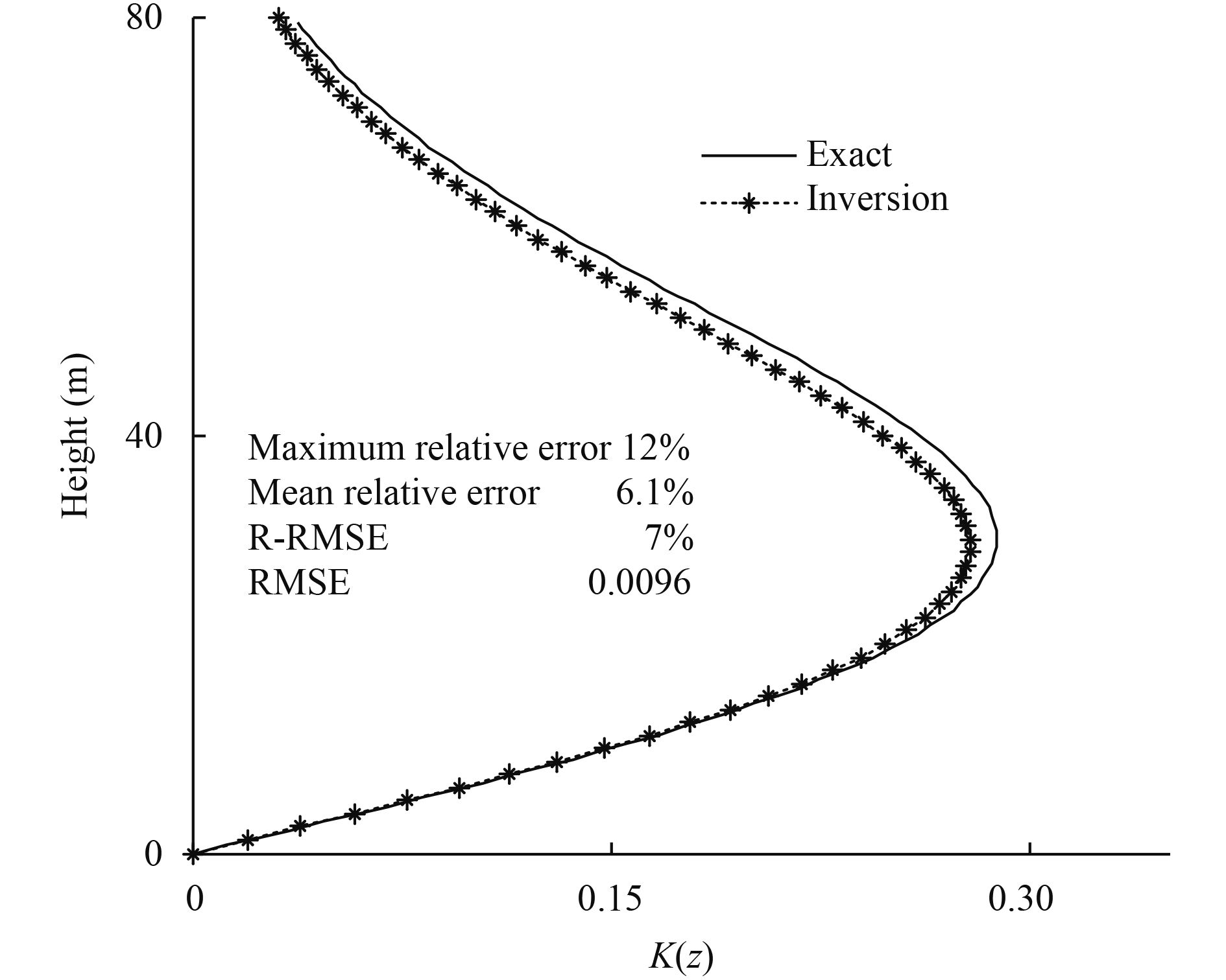
| Figure 5 Comparison between the inversion value of K(z) (dashed line with asterisks) and the exact value (solid line) under the condition of observation with noise. The coordinates and parameter are the same as in Fig. 3, so are the boundary conditions. The only difference between the experiments depicted in Figs. 3 and 5 is the observation data. |
We use the observations of wind speed and potential temperature with errors to retrieve the parameter K(z). The retrieved profiles of K(z) are shown in Fig. 5. In Fig. 5, the mean relative error is 6.1%; the maximum relative error is 12%; R-RMSE is 7%; and RMSE is 0.0096. These numbers indicate that the variational assimilation scheme we used has decently restrained the influence of the observation error. Therefore, we conclude that the proposed method is capable of accommodating the observation noises and suitable to retrieve the parameter in the weakly nonlinear Prandtl model with observation errors.
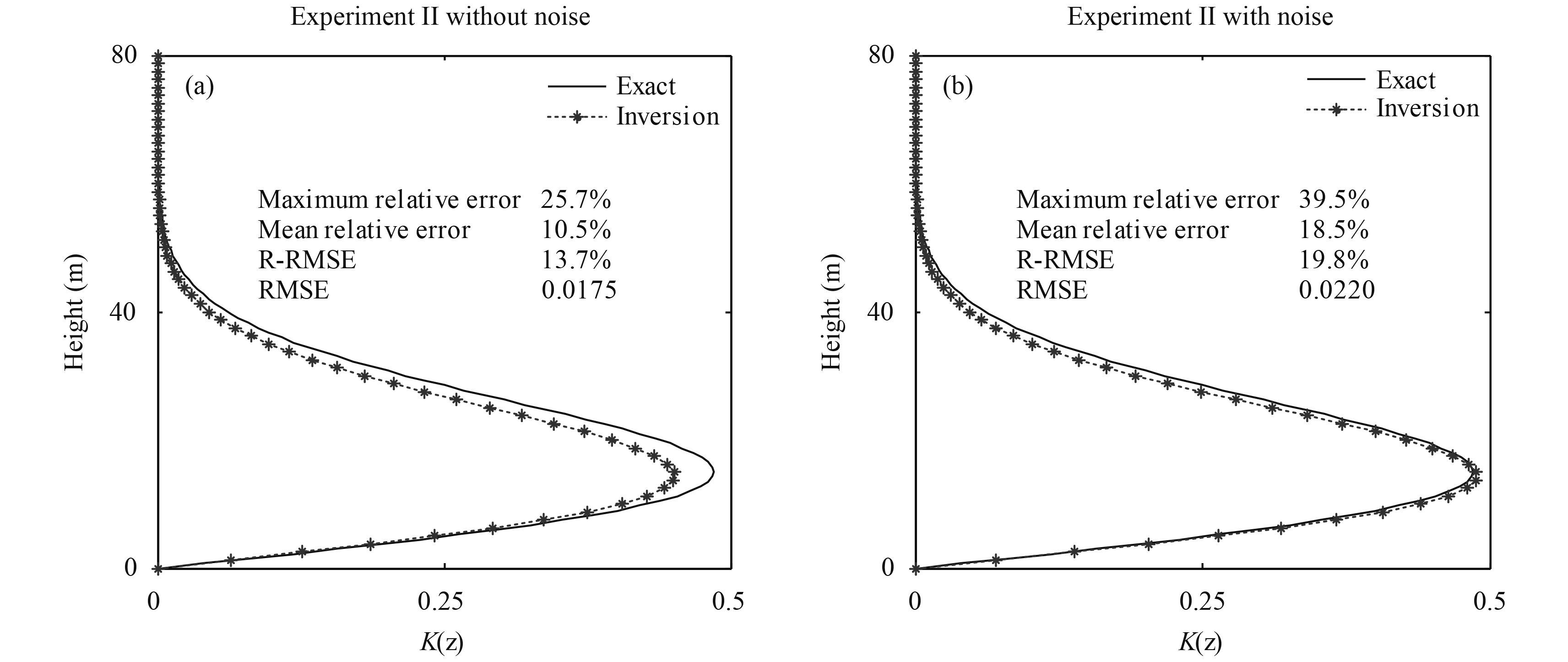
4.2 Experiment ⅡIt is expected that an increase in the number of samples should make the variational assimilation scheme more persuasive. In this experiment, we assume that
|
| Figure 6 Comparison between the inversion value of K(z) (dashed line with asterisks) and the exact value (solid line) for the retrieval (a) without observation noise and (b) with observation noise. The solid line represents the exact value and the dashed line with asterisks represents the inversion value of K(z). |
|
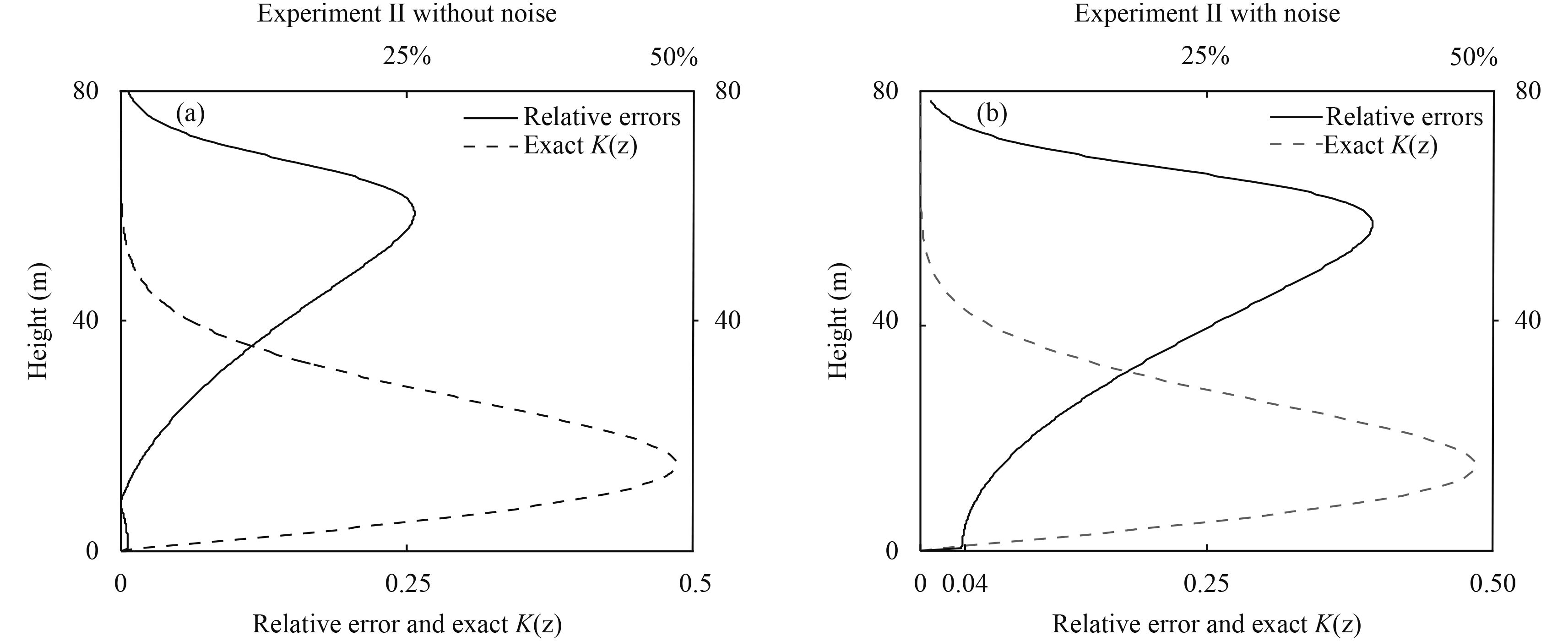
| Figure 7 Distribution of the relative error and exact K(z) with height for the retrieval (a) without observation noise and (b) with observation noise. The horizontal coordinate gives values of the exact eddy thermal conductivity and relative error. The solid line denotes the distribution of relative error with height. The dashed line indicates the distribution of exact eddy thermal conductivity with height. |
The error distribution with height is shown in Fig. 7. The maximum relative error of the retrieval without observation noise is 25.7% and the mean relative error is 10.5% (Fig. 7a). Meanwhile, the relative error below 40 m is less than 10%, and the R-RMSE and RMSE is 13.7% and 0.0175, respectively (Fig. 7a). The maximum relative error of the retrieval with observation noise is 39.5%; the mean relative error is 18.5%; the relative error below 40 m is less than 20%; the R-RMSE is 19.8%; the RMSE is 0.022; and the maximum absolute error is 0.04 (Fig. 7b). The maximum relative errors appear in the upper part of both Fig. 7a and Fig. 7b, where exact eddy thermal conductivities are close to zero. The large relative errors above 40 m seem to be associated with small K(z) values at zero and its vicinity.
5 Conclusions and discussionResearch on the slope flows in the atmospheric boundary layer has been a popular field in atmospheric sciences. Research on katabatic flows provides guidance to the development of weather and climate prediction models. The weakly nonlinear Prandtl model is more efficient than the classical Prandtl model as it introduces the small parameter
Research on inversion problems tells us that obtaining a retrieval model parameter is an ill-posed problem. It is more difficult to retrieve the K(z) without a fixed form. If we want to obtain the vertical distribution of K(z), we must obtain the statistical background information of K(z) first, and then use the variational regularization method to solve K(z). The WKB method is selected in this paper, and the solution is only an approximate one. Further study of direct numerical calculation is required.
Acknowledgments. We thank Professor Branko Grisogono for the PASTEX-94 dataset. We also thank the reviewers and Editor Xiaoming Hu for their constructive criticism that contributes to significant improvements to the original manuscript and greater reliability in interpretation of the numerical experiment results.
AppendixThis appendix contains the details of the WKB calculation steps. The weakly nonlinear Prandtl model is expressed as follows (meaning of each expression is the same as detailed in Section 2):
| $\begin{split}& g\frac{\theta }{{{\Theta _{\rm{0}}}}}\sin (\alpha) + K\Pr \frac{{{\partial ^2}u}}{{\partial {z^2}}} = 0, \\& - (\Gamma + \varepsilon \frac{{\partial \theta }}{{\partial z}})u\sin (\alpha) + K\frac{{{\partial ^2}\theta }}{{\partial {z^2}}} = 0.\end{split}$ | (A1) |
The expression of the global expansion of
| $\begin{array}{l}u = {u_0} + \varepsilon {u_1} + \varepsilon u_2^2 + \cdot \cdot \cdot, \\\theta = {\theta _0} + \varepsilon {\theta _1} + \varepsilon \theta _2^2 + \cdot \cdot \cdot .\end{array}$ | (A2) |
Now, we substitute Eq. (A1) with Eq. (A2) and keep the expansion up to the first order:
| $\begin{align} & g\frac{{{\theta }_{0}}}{{{\Theta }_{\text{0}}}}\sin (\alpha )+K\Pr \frac{{{{\rm d}}^{2}}{{u}_{0}}}{{\rm d}{{z}^{2}}} \\ \quad & +\varepsilon (g\frac{{{\theta }_{1}}}{{{\Theta }_{\text{0}}}}\sin (\alpha )+K\Pr \frac{{{{\rm d}}^{2}}{{u}_{1}}}{{\rm d}{{z}^{2}}})=0, \\ \quad & -\Gamma {{u}_{0}}\sin (\alpha )+K\frac{{{{\rm d}}^{2}}{{\theta }_{0}}}{{\rm d}{{z}^{2}}} \\ \quad & +\varepsilon (-(\Gamma {{u}_{1}}+\frac{{\rm d}{{\theta }_{0}}}{{\rm d}z}{{u}_{0}})\sin (\alpha )+K\frac{{{{\rm d}}^{2}}{{\theta }_{1}}}{{\rm d}{{z}^{2}}})=0. \\ \end{align}$ | (A3) |
A1. Zero-order expansion
The zero-order expansion reads
| $\begin{split}& g\frac{{{\theta _0}}}{{{\Theta _{\rm{0}}}}}\sin (\alpha) + K\Pr \frac{{{{\rm d}^2}{u_0}}}{{{\rm d}{z^2}}} = 0, \\ & - \Gamma {u_0}\sin (\alpha) + K\frac{{{{\rm d}^2}{\theta _0}}}{{{\rm d}{z^2}}} = 0.\end{split}$ | (A4) |
System (A4) can be rewritten to a single governing equation of the fourth order by the elimination method. The terms dK/dz and
As
| $\frac{{{{\rm d}^4}({u_0}, {\theta _0})}}{{{\rm d}{z^4}}} + {N^2}\frac{{{{\sin }^2}(\alpha)}}{{\Pr K\!{{(z)}^2}}}({u_0}, {\theta _0}) = 0.$ | (A5) |
If
| $\begin{array}{l}{u_0} = - C\mu \exp (- \frac{z}{{{h_{\rm p}}}})\sin (\frac{z}{{{h_{\rm p}}}}), \\{\theta _0} = C\exp (- \frac{z}{{{h_{\rm p}}}})\cos (\frac{z}{{{h_{\rm p}}}}), \end{array}$ | (A6) |
where C is the surface potential temperature deficit in the case of katabatic flows. The opposite, C < 0, is the temperature surplus, for anabatic flows. The parameter
If K(z) is the gradually varying term in Eq. (A5), then the argument in Eq. (A6),
| $I(z) = {({\sigma _0}/2)^{\frac{1}{2}}}\int_0^z {K\!{{(z)}^{ - \frac{1}{2}}}{\rm d}z}, $ | (A7) |
where σ0 is a factor in I (z) and
| $\begin{array}{l}{u_0} = - C\mu \exp (- I)\sin (I), \\{\theta _0} = C\exp (- I)\cos (I).\end{array}$ | (A8) |
Note that the term
A2. First-order correction
Next, the first-order correction is analyzed. The corresponding system at the order of ε1 is
| $\begin{split}& g\frac{{{\theta _1}}}{{{\Theta _0}}}\sin (\alpha) + K\Pr \frac{{{{\rm d}^2}{u_1}}}{{{\rm d}{z^2}}} = 0, \\& - (\Gamma {u_1} + \frac{{{\rm d}{\theta _0}}}{{{\rm d}z}}{u_0})\sin (\alpha) + K\frac{{{{\rm d}^2}{\theta _1}}}{{{\rm d}{z^2}}} = 0.\end{split}$ | (A9) |
The unknowns are
| $\begin{array}{l}\frac{{{{\rm d}^4}{u_1}}}{{{\rm d}{z^4}}} + {N^2}\frac{{{{\sin }^2}(\alpha)}}{{\Pr K\!{{(z)}^2}}}{u_1} = - \frac{{g{{\sin }^2}(\alpha)}}{{{\Theta _0}K\!{{(z)}^2}\Pr }}{u_0}\frac{{{\rm d}{\theta _0}}}{{{\rm d}z}}, \\\frac{{{{\rm d}^4}{\theta _1}}}{{{\rm d}{z^4}}} + {N^2}\frac{{{{\sin }^2}(\alpha)}}{{\Pr K\!{{(z)}^2}}}{\theta _1} = \frac{{\sin (\alpha)}}{{K\!(z)}}\frac{{{{\rm d}^2}}}{{{\rm d}{z^2}}}({u_0}\frac{{{\rm d}{\theta _0}}}{{{\rm d}z}}).\end{array}$ | (A10) |
Equation (A10) comprises inhomogeneous ordinary differential equations whose solutions consist of a general solution and a special solution; the knowns are
| $\begin{aligned}{u_1} & = {u_A}\exp (- I)[ - \frac{1}{3}\sin (I) + \frac{2}{{15}}\cos (I)]\\ & + {u_A}\exp (- 2I)[\frac{1}{{30}}\sin (2I) - \frac{1}{{30}}\cos (2I) - \frac{1}{{10}}], \\ {\theta _1} & = {\theta _A}\exp (- I)[ - \frac{1}{{15}}\sin (I) - \frac{1}{6}\cos (I)] \quad \quad \quad (\rm {A}11)\\ & + {\theta _A}\exp (- 2I)[\frac{1}{{15}}\sin (2I) + \frac{1}{{15}}\cos (2I) + \frac{1}{{10}}].\end{aligned}$ |
Here,
Thus, the total WKB approximate solutions, up to the first order, are as follows:
| $\begin{array}{l}u = {u_0} + \varepsilon {u_1}, \\\theta = {\theta _0} + \varepsilon {\theta _1}.\end{array}$ |
| Arnold, C. P., and Jr, and C. H. Dey, 1986: Observing-systems simulation experiments: Past, present, and future. Bull. Amer. Meteor. Soc., 67, 687–695. DOI:10.1175/1520-0477(1986)067<0687:OSSEPP>2.0.CO;2 |
| Axelsen, S. L., and H. van Dop, 2009: Large-eddy simulation of katabatic winds. Part 2: Sensitivity study and comparison with analytical models. Acta Geophys., 57, 837–856. DOI:10.2478/s11600-009-0042-5 |
| Baklanov, A. A., B. Grisogono, R. Bornstein, et al., 2011: The nature, theory, and modeling of atmospheric planetary boundary layers. Bull. Amer. Meteor. Soc., 92, 123–128. DOI:10.1175/2010BAMS2797.1 |
| Barthélemy, A., H. Goosse, P. Mathiot, et al., 2012: Inclusion of a katabatic wind correction in a coarse-resolution global coupled climate model. Ocean Modell., 48, 45–54. DOI:10.1016/j.ocemod.2012.03.002 |
| Buzzi, M., M. W. Rotach, M. Holtslag, et al., 2011: Evaluation of the COSMO-SC turbulence scheme in a shear-driven stable boundary layer. Meteor. Z., 20, 335–350. DOI:10.1127/0941-2948/2011/0050 |
| De Ridder, K., D. Lauwaet, and B. Maiheu, 2015: UrbClim—A fast urban boundary layer climate model. Urban Climate, 12, 21–48. DOI:10.1016/j.uclim.2015.01.001 |
| Denby, B., 1999: Second-order modeling of turbulence in kata-batic flows. Bound.-Layer Meteor., 92, 65–98. DOI:10.1023/A:1001796906927 |
| Egger, J., 1990: Thermally forced flows: Theory. Atmospheric Processes over Complex Terrain. Blumen W., Ed. Boston, MA, Amer. Meteor. Soc., 43–58. |
| Epifanio, C. C., 2007: A method for imposing surface stress and heat flux conditions in finite-difference models with steep terrain. Mon. Wea., Rev., 135, 906–917. DOI:10.1175/MWR3297.1 |
| Gao, J. D., C. J. Qiu, and J. F. Chou, 1995: The sensitivity influence of numerical model initial values on four-dimensional assimilation—Study based on Lorenz system. Acta Meteor. Sinica, 9, 278–287. |
| Grisogono, B., 2003: Post-onset behaviour of the pure katabatic flow. Bound.-Layer Meteor., 107, 157–175. DOI:10.1023/A:1021511105871 |
| Grisogono, B., and J. Oerlemans, 2001a: Katabatic flow: Analytic solution for gradually varying eddy diffusivities. J. Atmos. Sci., 58, 3349–3354. DOI:10.1175/1520-0469(2001)058<3349:KFASFG>2.0.CO;2 |
| Grisogono, B., and J. Oerlemans, 2001b: A theory for the estimation of surface fluxes in simple katabatic flows. Quart. J. Roy. Meteor. Soc., 127, 2725–2739. DOI:10.1002/qj.49712757811 |
| Grisogono, B., and J. Oerlemans, 2002: Justifying the WKB approximation in pure katabatic flows. Tellus, 54, 453–463. DOI:10.3402/tellusa.v54i5.12166 |
| Grisogono, B., and S. L. Axelsen, 2012: A note on the pure katabatic wind maximum over gentle slopes. Bound.-Layer Meteor., 145, 527–538. DOI:10.1007/s10546-012-9746-1 |
| Grisogono, B., T. Jurlina, Ž. Večenaj, et al., 2015: Weakly nonlinear Prandtl model for simple slope flows. Quart. J. Roy. Meteor. Soc., 141, 883–892. DOI:10.1002/qj.2406 |
| Hu, X. M., F. Q. Zhang, and J. W. Nielsen-Gammon, 2010: Ensemble-based simultaneous state and parameter estimation for treatment of mesoscale model error: A real-data study. Geophys. Res. Lett., 37, L08802. DOI:10.1029/2010GL043017 |
| Huang, S. X., J. Xiang, H. D. Du, et al., 2005: Inverse problems in atmospheric science and their application. J. Phys. Conf. Ser., 12, 45–57. DOI:10.1088/1742-6596/12/1/005 |
| Huang, S. X., X. Q. Cao, H. D. Du, et al., 2006: Retrieval of atmospheric and oceanic parameters and the relevant numerical calculation. Adv. Atmos. Sci., 23, 106–117. DOI:10.1007/s00376-006-0011-8 |
| Ingel, L. K., 2011: Toward a nonlinear theory of katabatic winds. Fluid Dyn., 46, 505–513. DOI:10.1134/S0015462811040016 |
| Jeričević, A., L. Kraljević, B. Grisogono, et al., 2010: Parameterization of vertical diffusion and the atmospheric boundary la-yer height determination in the EMEP model. Atmos. Chem. Phys., 10, 341–364. DOI:10.5194/acp-10-341-2010 |
| Kaipio, J., and E. Somersalo, 2005: Statistical and Computational Inverse Problems. Springer, 357 pp. |
| Lorenc, A. C., 1988: A practical approximation to optimal four-dimensional objective analysis. Mon. Wea. Rev., 116, 730–745. DOI:10.1175/1520-0493(1988)116<0730:APATOF>2.0.CO;2 |
| Mahrt, L., 1982: Momentum balance of gravity flows. J. Atmos. Sci., 39, 2701–2711. DOI:10.1175/1520-0469(1982)039<2701:MBOGF>2.0.CO;2 |
| Mahrt, L., 1998: Stratified atmospheric boundary layers and breakdown of models. Theoret. Comput. Fluid Dyn., 11, 263–279. DOI:10.1007/s001620050093 |
| Mo, R. P., 2013: On adding thermodynamic damping mechanisms to refine two classical models of katabatic winds. J. Atmos. Sci., 70, 2325–2334. DOI:10.1175/JAS-D-12-0256.1 |
| Navon, I. M., 1998: Practical and theoretical aspects of adjoint parameter estimation and identifiability in meteorology and oceanography. Dyn. Atmos. Oceans, 27, 55–79. DOI:10.1016/S0377-0265(97)00032-8 |
| Nielsen-Gammon, J. W., X. M. Hu, F. Q. Zhang, et al., 2010: Evaluation of planetary boundary layer scheme sensitivities for the purpose of parameter estimation. Mon. Wea. Rev., 138, 3400–3417. DOI:10.1175/2010MWR3292.1 |
| Salvador, N., N. C. Reis Jr, J. M. Santos, et al., 2016: Evaluation of weather research and forecasting model parameterizations under sea-breeze conditions in a North Sea coastal environment. J. Meteor. Res., 30, 998–1018. DOI:10.1007/s13351-016-6019-9 |
| Shapiro, A., B. Burkholder, and E. Fedorovich, 2012: Analytical and numerical investigation of two-dimensional katabatic flow resulting from local surface cooling. Bound.-Layer Meteor., 145, 249–272. DOI:10.1007/s10546-011-9685-2 |
| Shapiro, A., E. Fedorovich, and S. Rahimi, 2016: A unified theory for the Great Plains nocturnal low-level jet. J. Atmos. Sci., 73, 3037–3057. DOI:10.1175/JAS-D-15-0307.1 |
| Smith, C. M., and E. D. Skyllingstad, 2005: Numerical simulation of katabatic flow with changing slope angle. Mon. Wea. Rev., 133, 3065–3080. DOI:10.1175/MWR2982.1 |
| Stiperski, I., I. Kavčič, B. Grisogono, et al., 2007: Including Coriolis effects in the Prandtl model for katabatic flow. Quart. J. Roy. Meteor. Soc., 133, 101–106. DOI:10.1002/qj.19 |
| Sun, J. L., D. H. Lenschow, L. Mahrt, et al., 2013: The relationships among wind, horizontal pressure gradient, and turbulent momentum transport during CASES-99. J. Atmos. Sci., 70, 3397–3414. DOI:10.1175/JAS-D-12-0233.1 |
| Tan, Z. M., J. Fang, and R. S. Wu, 2006: Nonlinear Ekman layer theories and their applications. Acta Meteor. Sinica, 20, 209–222. |
| Tosaka, N., K. Onoshi, and M. Yamamoto, 1999: Mathematical Approach and Solution Methods for Inverse Problems: Inverse Analysis of Partial Differential Equation. University of Tokyo Press, 294 pp. (in Japanese) |
| van den Broeke, M. R., 1997: Structure and diurnal variation of the atmospheric boundary layer over a mid-latitude glacier in summer. Bound.-Layer Meteor., 83, 183–205. DOI:10.1023/A:1000268825998 |
| Yan, B., and S. X. Huang, 2014: Variational regularization me-thod of solving the Cauchy problem for Laplace’s equation: Innovation of the Grad–Shafranov (GS) reconstruction. Chinese Phys. B, 23, 650–655. DOI:10.1088/1674-1056/23/10/109402 |
| Zhao, X. F., and S. X. Huang, 2012: Estimation of atmospheric duct structure using radar sea clutter. J. Atmos. Sci., 69, 2808–2818. DOI:10.1175/JAS-D-12-073.1 |
 2017, Vol. 31


