 2016, Vol. 30
The Chinese Meteorological Society
Article Information
- SHEN Lidu, SUN Jianning, YUAN Renmin, LIU Peng . 2016.
- Characteristics of Secondary Circulations in the Convective Boundary Layer over Two-Dimensional Heterogeneous Surfaces. 2016.
- J. Meteor. Res., 30(6): 944-960
- http://dx.doi.org/10.1007/s13351-016-6016-z
Article History
- Received February 16, 2016
- in final form July 17, 2016


2. (State Key Laboratory of Severe Weather, Chinese Academy of Meteorological Sciences, Beijing 100081);
3. (Longquanyi District Meteorological Service of Chengdu, Chengdu 610100);
The heterogeneity of the land surface can impose considerable effects on turbulence characteristics of the atmospheric boundary layer (ABL) and its development (Shen and Leclerc, 1995; Avissar and Schmidt, 1998; Raasch and Harbusch, 2001; Letzel and Raasch, 2003; Kang and Davis, 2008; Kang, 2009; Liu et al., 2011; Maronga and Raasch, 2013; Kang and Lenschow, 2014; Sühring et al., 2014). The secondary circulations (SCs) induced by the surface heterogeneity can significantly affect the transport of heat, mass, and humidity, and even the formation of clouds and precipitation (Ookouchi et al., 1984; Segal et al., 1988; André et al., 1990; Chen and Avissar, 1994; Liu and Avissar, 1996; Patton et al., 2005; Courault et al., 2007; van Heerwaarden and de Arellano, 2008; van Heerwaarden et al., 2009; Ouwersloot et al., 2011). Accurate descriptions of the heterogeneity-influenced boundary layer will help to improve the performance of weather forecast models. However, uncertainties and nonlinear processes induced by the heterogeneous land surface range from the mesoscale down to the microscale, and their effects on the ABL have not been fully investigated yet (Maronga and Raasch, 2013). Since the heterogeneity-induced effects can barely be captured by field measurements, turbulence-resolving large-eddy simulations (LESs) have been employed to investigate the interaction between the surface heterogeneity and the convective boundary layer (CBL). In most of the studies mentioned above, the land surface was specified with ideal one-dimensional (1D stripelike) or two-dimensional (2D chessboard pattern) variation of surface heat flux, soil moisture, etc. The results of these studies show that the turbulence characteristics in the CBL are influenced by the heterogeneity length scale and amplitude, and also affected by wind speed and wind direction.
Many LESs have been conducted with 1-D heterogeneous surface forcing (e.g., Avissar and Schmidt, 1998; Patton et al., 2005; Kang and Davis, 2008; Kang, 2009; Ouwersloot et al., 2011; Sühring et al., 2014). Ouwersloot et al. (2011) and Sühring et al. (2014) found that the largest entrainment occurs when the patch size is about one to two times zi (meaning that the heterogeneity length scale, λ, is about two to four times zi, where zi is the boundary layer height). For the influence of background wind, previous studies have reported that when the wind is perpendicular to the border between the differently-heated patches, the SCs are depressed; when the wind is parallel to the border between the patches, the SCs are triggered (Avissar and Schmidt, 1998; Kim et al., 2004; Ouwersloot et al., 2011; Sühring et al., 2014). There are relatively fewer studies on the effect of 2D surface heterogeneities on the SCs. Raasch and Harbusch (2001) reported that when the wind blows parallel to the side of the chessboard pattern, the impact of surface heterogeneity is considerably reduced under a weak background wind of 2.5 m s-1. However, when the wind direction is along the diagonal of the chessboard pattern, the roll-like SCs develop with their roll axes orientated along the mean wind direction and persist even under a larger background wind speed of 7.5 m s-1. Courault et al. (2007) used an LES model coupled with a soil vegetation atmosphere transfer model to investigate the feedback of surface sensible and latent heat fluxes to the heterogeneity-induced SCs. Liu et al. (2011) found that the SCs in a shear-free CBL break up at a certain time when λ/zi becomes small enough due to the increased boundary layer height. Maronga and Raasch (2013) carried out LESs over irregular 2D heterogeneous surfaces. They found that the SC patterns vary between local and roll-like structures, depending on the background wind condition. Kang and Lenschow (2014) investigated the influence of 2D mesoscale surface heat-flux heterogeneity (λ=32 km) on low-level winds in the CBL. They found that with a background wind of 5 m s-1, the heterogeneity-induced mesoscale circulations are somewhat stronger than those with no background wind.
So far, studies on the effects of 2D surface heterogeneity are less than sufficient. However, the real land surface usually exhibits a feature of 2D heterogeneity, for example, cropland. This study aims to investigate the effect of a 2D heterogeneous surface on the CBL structure under varying conditions of heterogeneity scale and wind speed. While several previous studies have suggested that the strongest impact of 1D surface heterogeneity occurs on the heterogeneity scale of about two to four times zi (Ouwersloot et al., 2011; Sühring et al., 2014), their results were obtained by comparing outputs from different cases when the CBLs have the same height. Details of the continuous variation of SC intensity are still unknown. Liu et al. (2011) reported that the 2D heterogeneity-induced SCs break up when there is no background wind, while Maronga and Raasch (2013) found that the SCs do not break up when background winds exist. Therefore, this study focuses on the evolution of turbulence characteristics and SC intensity during CBL development, and investigates whether a threshold exists for the SCs to break up and, if so, what the threshold is in the 2D heterogeneous case. Different LESs are conducted to evaluate the influences of different heterogeneity length scales and background wind speeds on the turbulence characteristics and SC structure in the CBL over the 2D heterogeneous surface.
2Methods 2.1Model descriptionA suite of numerical experiments has been conducted by using the Dutch Atmospheric Large-Eddy Simulation (DALES) model, which was updated to a parallel version by Dosio (2005). By applying the Boussinesq approximation, the DALES model solves the filtered Navier-Stokes equations (Heus et al., 2010). It is run on an Arakawa Cgrid. The time integration is performed by a third-order Runge-Kutta scheme and an adaptive time-step is applied for efficient integration. The model uses a fifth-order advection scheme following Wicker and Skamarock (2002). The subgrid-scale processes are parameterized by the 1.5-order turbulent kinetic energy (TKE) closure (Deardorff, 1980). Monin-Obukhov similarity theory is employed at the lowest model level to calculate the surface momentum flux. The lateral boundary conditions are periodic. Fluctuations of velocity and scalars due to gravity waves are damped out by a sponge layer in the upper part of the domain.
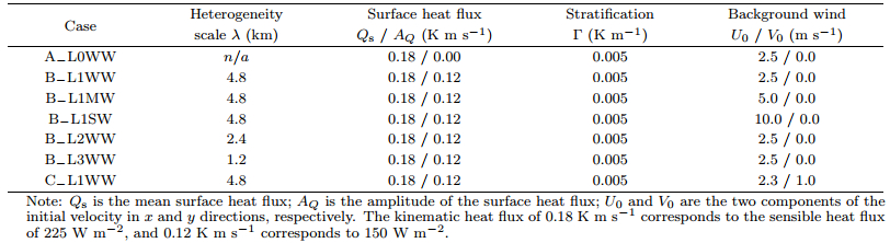
2.2Experimental setupThe model domain is 9.6 km × 9.6 km × 4.0 km. The cell length is 50 m in the x and y directions and 10 m in the z direction. The horizontal grid length is the same as that in Ouwersloot et al. (2011). The sensitivity experiments in Sullivan and Patton (2011) showed that this resolution can describe the turbulence statistics and the entrainment process well. The patterns of surface heat flux distribution are illustrated in Fig. 1. A mean surface kinematic heat flux of 0.18 K m s-1 with an amplitude of 0.12 K m s-1 is prescribed in the heterogeneous cases. For the purpose of comparison, one homogeneous case named A_L0WW is also conducted. The cases in which the wind direction is along the diagonal of the chessboard pattern are named starting with the letter “B”. In order to know how and where the SCs develop when the wind is not along the diagonal of the chessboard pattern, another case in which the wind direction is 22.5° relative to the chessboard side is conducted and named starting with the letter “C”. Previous studies have demonstrated that the SCs are suppressed when the wind direction is orientated along the side of the chessboard pattern. This situation is not considered in this study. The heterogeneity length scale is denoted by the following two letters. “L1”, “L2”, and “L3” denote that λ is 4.8, 2.4, and 1.2 km, respectively. The background wind speed is denoted by the last two letters. “WW”, “MW”, and “SW” represent weak wind (2.5 m s-1), moderate wind (5 m s-1), and strong wind (10 m s-1), respectively. Our simulations show that in the cases with the two small heterogeneity length scales, the SCs break down during the CBL development under weak background wind (the results are presented in Section 3.3). Therefore, we only discuss the effect of wind speed on the SC characteristics for the cases with the largest heterogeneity length scale. Configurations for these simulations are listed in Table 1.

|
| Figure 1 Distributions of heterogeneous surface heating for the cases of (a) A_L0WW; (b) C_L1WW, C_L1MW, and C_L1SW; (c) C_L2WW; (d) C_L3WW; and (e) C_L1WW. Black, grey, and white colors represent the heat flux values of 0.06, 0.18, and 0.3 K m s-1, respectively. The arrow on top-right of each subplot indicates the wind direction. |
All simulations have the same initial potential temperature profile with a lapse rate of 0.005 K m-1 and 300 K at the ground. To keep the wind direction unchanged, the background wind is imposed by the initial wind speed at all grid points in the atmosphere and the Coriolis force is neglected. This treatment is the same as in Raasch and Harbusch (2001). A dry CBL is assumed. The surface roughness length is set to be 0.1 m. To investigate the evolution of turbulence characteristics and SCs in the CBL, the simulations cover a period of 10 h. The three-dimensional output data are saved every 5 minutes. The outputs after the first hour, which is usually regarded as the spin-up time, are used for analysis. In this study, the spin-up time is associated with the formation of the equilibrium state of the SCs since there is no initial constant potential temperature layer. In other words, the CBL over the heterogeneous surface should reach the state that the dominant horizontal scale of the turbulent eddies is the same as the surface heterogeneity length scale. The results in Liu et al. (2011) indicated that under no background wind condition, the case with λ=10 km needs a spin-up time of 1.5 h, while the case with λ=5 km needs a spin-up time less than 1 h. Our simulations show that the background wind is favorable for the SC development (the results are given in Section 3.3). Therefore, in all of our cases the spin-up time is shorter than 1 h.
It should be noted that the side width of the squares in C_L1WW is not 4.8 km. However, the results in Maronga and Raasch (2013) indicated that the flow responds to an effective heat-flux pattern that derives from the original pattern by streamwise averaging. For the case C_L1WW, averaging the surface heat flux along the x or y direction results in a heterogeneity length scale of 4.8 km in the y or x direction. Consequently, the heterogeneity length scales in C_L2WW and C_L3WW are 2.4 and 1.2 km, respectively. The LES results show that the SC structure in C_L1WW is similar to that in C_L1WW. Thus, its heterogeneity scale is also 4.8 km.
2.3Statistical analysisThe boundary layer height, zi, is defined as the height at which the horizontally domain-averaged heat flux reaches the minimum value. The entrainment flux ratio, Ae, is defined as

|
(1) |
where 

According to the above definition, an irregular physical quantity f can be decomposed into two parts:

|
(2) |
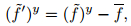
where f is the horizontal average of f, which can be a velocity component (u, v, w) or potential temperature (θ) in this study; f' is the deviation from the horizontal average (i.e., u', v', w', or θ'). The velocity variances (σu2, σv2, and σw2) are calculated from u', v', and w', and the potential temperature variance (σθ2) is calculated from θ'. When the irregular quantity f is av eraged across the domain in the x or y direction, the obtained 


|
(3) |
and
|
(4) |
where the wave-bar denotes the direction-average, and the superscript denotes that the averaging is operated along the x or y direction.
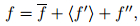
In this study, phase-average analysis is also applied. According to previous studies (Shen and Leclerc, 1995; Raasch and Harbusch, 2001; Patton et al., 2005; Maronga and Raasch, 2013), any irregular physical quantity f can be decomposed into three components:
|
(5) |
where f is the horizontal average component, 〈f'〉 is the heterogeneity-induced (phase-correlated) component, and f" is the random component (the background turbulence). The two dimensional phase coordinate system 


In this study, the background wind is specified by the initial wind field rather than the geostrophic wind, and there is no horizontal forcing for the simulations of flows. The mean wind maintains during the CBL development due to the downward transfer of momentum from above the CBL to the interior CBL. This situation may somewhat differ from that when the geostrophic wind and the Coriolis force both exist. The LES outputs show that the mean velocity is approximately constant with height in the mixed layer, but changes sharply across the CBL top and remains unchanged in the free atmosphere. This is the typical shape of the profile of mean velocity in a CBL, as reported in the classical book An Introduction to Boundary Layer Meteorology (Stull, 1988). The LES outputs also exhibit typical vertical distributions of the mean potential temperature and heat flux in the CBL, which agree well with those reported in previous studies (e.g., Raasch and Harbusch, 2001; van Heerwaarden and de Arellano, 2008; Ouwersloot et al., 2011; Maronga and Raasch, 2013; Sühring et al., 2014). These results suggest that the simulated CBLs have reasonable vertical structures.
The LES outputs show that the profiles of σu2, σv2, and σw2 in cases C_L1WW and C_L1WW are the same as the results in Raasch and Harbusch (2001). The vertical distribution of v-variance in the heterogeneous cases displays a two-peak feature. The two peaks are located in the surface layer and the upper mixed layer, respectively, corresponding to the lower and upper branches of the triggered SCs in the crosswind direction. The turbulence characteristics in C_L1WW have rarely been reported in previous studies. Figure 2 gives the cross-sections of the velocity and potential temperature perturbations that are obtained by averaging the perturbations along the x or y direction across the domain. There is no SC in the homogeneous case. In the case C_L1WW, the detected SCs in the x-z cross-section are very weak and the shape of these SCs is very vague (Fig. 2c). However, the roll-like SCs are triggered and develop vigorously in the y-z cross-section (Fig. 2d). This is because the strong (or weak) heating patches are linked together by the wind, leading to a stripe-like distribution (shown in Figs. 3d-f). Our results in C_L1WW support the argument in Maronga and Raasch (2013) that the flow feels an effective heat-flux pattern that derives from the original pattern by streamwise averaging, and the effective pattern generates the roll-like SCs with roll axes orientated along the mean wind direction.

|
| Figure 2 The (a, c, e) x-z and (b, d, f) y-z cross-sections of the direction-average velocity perturbations (curly vectors) and potential temperature perturbations (colors) at the simulation time of 3 h for (a, b) case A_L1WW, (c, d) case B_L1WW, and (e, f) case C_L1WW. The thick dashed line indicates the boundary layer height. |

|
| Figure 3 Horizontal cross-sections at the height of z=0.1zi for (a-c) case A_L1WW, (d-f) case B_L1WW, and (g-i) case C_L1WW at the simulation time (a, d, g) 1 h, (b, e, h) 3 h, and (c, f, i) 5 h. The color shadings represent perturbations of potential temperature, and vectors (curly vectors) represent perturbations of horizontal velocity. |
The SC structures in C_L1WW shown in Figs. 2e and 2f are quite similar to those in C_L1WW. The SC locations move downstream due to the advection of mean wind. The magnitude of the positive temperature perturbations (red areas) near the surface is smaller in C_L1WW than in C_L1WW, implying that the near-surface temperature gradient and consequently the horizontal pressure gradient are reduced by the wind component in the y direction. It should be noted that the wind direction in C_L1WW is not along the x axis. The surface heterogeneity along the wind direction in this case is more complex than in B_L1WW. Our calculations indicate that the variance of streamwise turbulent velocity is almost the same as the variance of the u-component turbulent velocity, while the variance of the spanwise turbulent velocity is always smaller than the variance of the v-component turbulent velocity (figures omitted), suggesting that the axes of the roll-like SCs are orientated along the x direction rather than along the mean wind direction.
Figure 2e shows stripe-like perturbations of pote-ntial temperature and velocity above the CBL, indicating a heterogeneous distribution along the x direction. Additionally, the stripes tilt toward the upstream direction. However, this phenomenon cannot be seen in Fig. 2f, implying that it is not a result of the advection of mean wind since the velocity component in the x direction is significantly larger than that in the y direction in case C_L1WW, and the strong smoothing effect of advection should eliminate the heterogeneity in the x direction. Further analysis suggests that this phenomenon is associated with the velocity component in the y direction, since this feature cannot be found in case B_L1WW (Fig. 2c), in which there is no v-component velocity. It is not clear why the combined condition in this case can trigger such stripe-like perturbations of potential temperature and velocity in the free atmosphere. This issue is beyond the scope of this study and will be investigated in our future work.
Figure 3 shows the perturbations of potential temperature and horizontal velocity at the height of z=0.1zi in the three cases at different times. In case A_L0WW, the distributions of temperature and horizontal velocity perturbations display random structures (Figs. 3a-c). In case C_L1WW, higher temperature appears over the central line of the aligned patches with high surface heat flux, while lower temperature appears over the patches with low surface heat flux. This pattern produces a horizontal temperature gradient and subsequently a pressure gradient in the crosswind direction, which induce horizontal motions towards the “warm line” and stimulate the development of roll-like SCs (Figs. 3d-f). In case C_L1WW, temperature perturbations and the turbulent velocities are somewhat more randomly distributed than in B_L1WW (Figs. 3g-i), implying that the roll-like SCs in this case are weaker than those in B_L1WW. For the two heterogeneous cases, the zones of enhanced perturbations aligned with the mean wind appear to weaken and become less organized in time, because the turbulent mixing enhances with continuous surface heating. These features coincide with the results shown later in Fig. 8 that the heterogeneity-induced near-surface temperature gradient in the y direction decreases with time and the decrease mainly occurs in the first half period of simulation.

|
| Figure 4 Horizontal cross-sections at the height of z=0.5zi for (a-c) case A_L1WW, (d-f) case B_L1WW, and (g-i) case C_L1WW at the simulation time (a, d, g) 1 h, (b, e, h) 3 h, and (c, f, i) 5 h. The color shadings represent the vertical velocity. The yellow lines represent the wind direction. |

|
| Figure 5 Time series of the (a, c, e) boundary-layer height and (b, d, f) entrainment flux ratio in different cases for (a, b) A_L0WW, B_L1WW, and C_L1WW; (c, d) A_L0WW, B_L1WW, B_L2WW, and B_L3WW; and (e, f) B_L1WW, B_L1MW, and B_L1SW. |

|
| Figure 6 Vertical profiles of the turbulence variances (solid lines) and the heterogeneity-induced perturbation variances (dashed lines) for (a-c) v-component and (d-f) w-component in cases B_L1WW and C_L1WW at the simulation time (a, d) 1 h, (b, e) 3 h, and (c, f) 5 h. |

|
| Figure 7 Temporal variations of (a) the heterogeneity-induced w-variance in cases B_L1WW, B_L2WW, and B_L3WW, (b) heterogeneity-induced w-variances, and (c) ratios of the heterogeneity-induced w-variance to the vertical turbulence velocity variance at z=0.5zi in cases B_L1WW, B_L1MW, and B_L1SW. The squares represent the hourly mean values. |

|
| Figure 8 (a) The phase-averaged and then x-directional-averaged near-surface temperature perturbation distribution in B_L1WW at different simulation times. (b) Temporal variations of the near-surface temperature gradient in cases B_L1WW, B_L1MW, and B_L1SW. The squares represent the hourly mean values. |
Figure 4 shows the vertical velocity distribution at the middle level of the CBL in the three cases at different times. It is not surprising that the upward motion in A_L0WW is distributed randomly (Figs. 4a-c). For case C_L1WW, the vertical motion displays a stripe-like distribution that is induced by the roll-like SCs (Figs. 4d-f). For case C_L1WW, Figs. 4g-i show that the distribution of the upward motion is approximately the same as in case C_L1WW, although the stripes are somewhat distorted. The displacement is caused by the wind component in the y direction. The stripes are not along the mean wind direction (the yellow lines) but along the x direction, indicating that the axes of roll-like SCs are orientated along the x direction. This result does not conflict with the findings in Maronga and Raasch (2013) that the flow feels an effective heat-flux pattern derived from the original pattern by streamwise averaging, and this effective pattern generates the roll-like SCs with roll axes orientated along the mean wind direction. Actually, in case C_L1WW the velocity component in the x direction is larger than that in the y direction, and the warm patches are linked in the x direction, as shown in Figs. 3g-i. Therefore, the roll-like SCs respond to the chessboard-like surface heating with their roll axes orientated in the direction along the diagonal with the larger velocity component, because both the warm patches and the cold patches are linked in this direction.
3.2The growth rate of CBL height in different casesFor the CBL, the convective velocity scale is defined as w 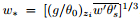

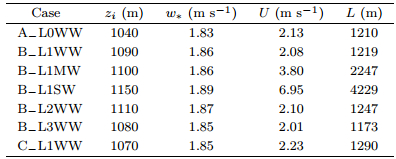
Figure 5a shows that the CBL in C_L1WW grows the fastest and has the highest height, while the CBL in C_L1WW grows faster than in A_L0WW but slower than in B_L1WW. The growth rate of boundary layer height (dzi/dt) is different in these cases, although the mean surface heat flux, background stratification, and wind speed are the same. The only difference between the heterogeneous cases is the wind direction. Therefore, the different growth rates of the CBL over the heterogeneous surface are caused by different wind directions.
The growth rate of the CBL is associated with the entrainment process at the CBL top, and the entrainment flux ratio Ae is usually used to characterize this process. Figure 5b shows that C_L1WW has the largest value of Ae. The value of Ae in C_L1WW is smaller than in C_L1WW but larger than in A_L0WW. Since the entrainment flux ratio is positively correlated with the growth rate of the CBL height, it is expected that the case with a larger entrainment flux ratio has a faster growth rate of the CBL height, and vice versa. Different values of Ae represent different characteristics of the entrainment process, which is associated with the turbulence characteristics in the CBL. The above results suggest that different entrainments are caused by different patterns of surface heterogeneity.
Figures 5c and 5d present the time series of CBL height and entrainment flux ratio in B-pattern cases with different patch sizes. The CBL height in B_L2WW is very close to that in C_L1WW. The details in their temporal variations, however, are different. The CBL growth rate in C_L2WW is slightly larger in the first half period of simulation, whereas it is slightly smaller in the second half period of simulation than in B_L1WW. This is consistent with the temporal variation of the entrainment flux ratio, which shows that the value of Ae in C_L2WW is larger than in B_L1WW in the first half period of simulation, and then begins to decrease and finally becomes smaller than in B_L1WW. The CBL growth rate in C_L3WW becomes smaller than in B_L1WW and C_L2WW after t=3 h. The value of Ae in C_L3WW also becomes smaller than in B_L1WW and C_L2WW after t=3 h. These results indicate that the entrainment process is different in the three cases. Apparently, the turbulence characteristics during the CBL development are influenced not only by the distribution pattern of surface heterogeneity, but also by the surface heterogeneity length scale.
Figures 5e and 5f show that there is no obvious difference in the CBL height between C_L1WW and B_L1MW, but the value of Ae in C_L1MW is slightly larger than in C_L1WW before t=4 h. The difference in the CBL growth rate is smaller than in the entrainment flux ratio. This is because the CBL growth rate is largely affected by the encroachment and is thus less sensitive to the variation of entrainment (Sühring et al., 2014). However, as the value of Ae in C_L1SW is obviously larger than in the other two cases before t=4 h, the CBL grows faster in C_L1SW than in the other two cases during the same period. But the CBL growth rate becomes smaller thereafter due to the decrease in entrainment flux ratio (although the value of Ae fluctuates significantly, an evident decreasing trend can still be seen after t=6 h). These results indicate that the increasing background wind speed tends to enhance the entrainment process, which is in agreement with the results of Raasch and Harbusch (2001). However, our results show that the enhancement of entrainment mainly occurs in the early hours of the CBL development.
Several previous studies have demonstrated that the background wind induces wind shear at the CBL top, which can enhance the entrainment process and promote the development of CBL over a homogeneous surface (Kim et al., 2003, 2006; Conzemius and Fedorovich, 2006, 2007; Pino et al., 2006; Sun and Xu, 2009). Note that in these studies the background wind is imposed by the geostrophic wind and the Coriolis force is considered. When the height-constant geostrophic wind speed is 10 m s-1, the increase in entrainment flux ratio is negligibly small compared to that in the case with no background wind (Sun and Xu, 2009). The background wind speed in our simulation cases is not larger than 10 m s-1. However, the entrainment flux ratio in the heterogeneous cases clearly increases (shown in Figs. 5b-d). The enhanced entrainment, especially in C_L1WW, is attributed to the effect of surface heterogeneity rather than the wind shear. Analyses in the next section show that the different characteristics in the temporal change of entrainment in these different cases are associated with the evolution of heterogeneity-induced roll-like SC intensity.
3.3Effects of the heterogeneity scale and wind speedThe results in last section have shown that the evolutions of the CBL height growth rate and the entrainment flux ratio in B_L2WW and C_L3WW are different from those in B_L1WW, suggesting that different surface heterogeneity length scales have different effects on the CBL turbulence. Here, we mainly discuss the influence of heterogeneity length scale on the SC characteristics. The heterogeneity-induced perturbations are analyzed. Figure 6 displays the heterogeneity-induced variances and total variances of v and w in B_L1WW and C_L1WW. They all increase with time. The increase in heterogeneity-induced w-variance with time indicates that the rolllike SCs intensify in the CBL developing process. The relatively small value of heterogeneity-induced wvariance in C_L1WW means that the SCs in this case are weaker than in B_L1WW.
As shown in Fig. 6, the maximum of the heterogeneity-induced w-variance occurs at the height of 0.5zi. Thus, we use [σw2 ]hi at 0.5zi to represent the SC intensity. Figure 7a shows that in C_L1WW, the SC intensity increases with time. However, in B_L2WW, the SC intensity increases in the first half period of simulation, but decreases in the second half, and finally becomes zero at the end of the simulation. In B_L3WW, the SC intensity decreases rapidly to almost zero before t=3 h. These results are in accordance with the evolutions of the entrainment flux ratio in these cases shown in Fig. 5d, implying that the entrainment process is associated with the SC intensity.
The horizontal length scale of large eddies is about 1.6 times the boundary layer height (Courault et al., 2007; Liu et al., 2011). In C_L2WW, the overturning time approximately occurs at t=5.5 h (Figure 7a), when the boundary layer height is about 1500 m (Fig. 5c). Thus, the horizontal scale of large eddies is 1.6zi=2400 m, which is equal to the heterogeneity length scale (λ=2.4 km). This means that the SC intensity begins to decrease at this moment, at which the scale of large eddies is the same as the heterogeneity length scale and then the turbulence characteristics become similar to those in the homogeneous case. In case B_L3WW, the boundary layer height is about 750 m at t=1.5 h (Fig. 5c), and the horizontal scale of large eddies is 1.6zi=1200 m, which is the heterogeneity length scale (λ=1.2 km). Figure 7a shows that the SC intensity in C_L3WW decreases rapidly after this moment. On the other hand, the SC intensity increases continuously in case C_L1WW, because the horizontal scale of large eddies (about 3.2 km) is still smaller than the heterogeneity length scale (4.8 km) at the end of the simulation. The results shown in Fig. 7a indicate that the roll-like SCs intensify when the heterogeneity length scale is larger than the horizontal scale of large eddies. However, the roll-like SCs are suppressed and finally break down once the heterogeneity length scale becomes smaller than the horizontal scale of large eddies. This result is different from that in Liu et al. (2011), who showed that the SCs would break down if the heterogeneity length scale is still larger than the horizontal scale of large eddies. The results of the present study suggest that weak wind (2.5 m s-1) is favorable for the development of roll-like SCs as long as the heterogeneity length scale is larger than the horizontal scale of large eddies. For the quite large heterogeneity length scale (λ=32 km) in Kang and Lenschow (2014), the SCs, therein called heterogeneity-induced mesoscale circulations, could be enhanced in the spanwise direction by the background wind.
Cases B_L1MW and C_L1SW are compared to B_L1WW to analyze the influence of wind speed on the roll-like SCs. The evolutions of [σw2]hi at the height of 0.5zi in the three cases are shown in Fig. 7b. The SC intensity in C_L1MW increases with time and is slightly larger than in C_L1WW, which is in good agreement with the result shown in Fig. 5f, which indicates that the entrainment flux ratio in B_L1MW is slightly larger than in C_L1WW, especially in the early hours of simulation. This result suggests that the SCs intensify somewhat under the moderate wind speed condition compared with that under the weak wind speed condition. The SC intensity in C_L1SW also increases with time, but the rate of increase is different from that in B_L1MW. It is larger during the first half period of the simulation but becomes smaller during the second half period than in C_L1WW. This situation corresponds with the changes in the entrainment flux ratio shown in Fig. 5f. These results suggest that the SCs are also intensified by the strong wind speed, but the intensification is more significant in the early hours of the CBL development. At t=1.5 h, C_L1SW has the largest SC intensity, C_L1WW has the smallest SC intensity, and the SC intensity in B_L1MW is between. As shown in Fig. 7c, [σw2]hi/σw2 in the three cases has the same order at t=1.5 h. This means that in the early stage of the CBL development a larger wind speed leads to stronger rolllike SCs. Subsequently, however, the growth rate of [σw2]hi/σw2in C_L1MW is significantly smaller than in B_L1WW, while the value of [σw2]hi/σw2in C_L1SW decreases with time. These results imply that more energy of vertical turbulent motion is distributed to the random turbulence during the CBL development under the condition of larger wind speed. This may be attributed to the larger shear-produced TKE induced by the larger wind speed.
The intensity of the vertical motion in the SCs is related to the temperature gradient near the ground. The phase-average method is first applied to the potential temperature at the lowest level in the atmosphere, and then the streamwise average is performed to obtain the surface potential temperature gradient. Figure 8a shows the results in C_L1WW at different times. At t=1 h, the surface potential temperature gradient is much greater than those at the other times. After t=4 h, the temperature gradient remains almost unchanged. The decrease in the temperature gradient results from the decrease in the maximum temperature 

In this study, DALES is employed to reproduce the CBL development over 2D heterogeneous surfaces. The distribution of heterogeneous surface heating is idealized to be a chessboard-like pattern. A suite of numerical experiments is conducted with varying heterogeneous length scale, wind speed, and wind direction to investigate the turbulence and SC characteristics in the CBL developing process under different conditions, and one homogeneous case is also conducted for comparison.
The cases with λ=4.8 km and U=2.5 m s-1 but with different wind directions are first compared with the homogeneous case. When the wind direction is parallel to the diagonal of the chessboard pattern (case C_L1WW), the roll-like SCs persist during the process of the CBL development, and the SC intensity increases with time. When the wind direction changes by 22.5° from the side of the chessboard pattern (case C_L1WW), the roll-like SCs can still be triggered, but the SC intensity is weaker than that in C_L1WW. The roll axes in C_L1WW are not orientated along the mean wind but along the x direction, implying that the diagonal of the chessboard pattern is the direction favorable for the development of the roll-like SCs over the 2D heterogeneous surface. This result indicates that the direction favorable for the SC development is the direction along which the averaged heat flux pattern (in the transverse direction) has the maximum amplitude. The chessboard pattern has two possible directions favorable for the SC development. Case C_L1WW indicates that the direction of the larger wind component is the actual direction favorable for the SC development. The results in C_L1WW extend the findings from previous studies.
Second, the effect of the heterogeneity length scale on the turbulence characteristics is also investigated. The three cases with different heterogeneity length scales suggest that an overturning moment for the rolllike SCs exists. Before this moment the SCs develop vigorously, and the SC intensity increases with time. After this moment the SCs are dampened and eventually break down. The overturning for the roll-like SCs occurs when the horizontal scale of large eddies beco-mes the same as the heterogeneous length scale, i.e., λ=1.6zi, during the CBL development. Our results suggest that a weak background wind is favorable for the maintaining of the SCs and the overturning of the roll-like SCs is related to a definite value of λ/zi.
Third, it is found in this study that a larger background wind speed can lead to a larger SC intensity in the early stage of the CBL development. As a result, the entrainment at the CBL top enhances and the growth rate of the CBL height increases. This is because the larger wind speed results in a larger surface temperature gradient, which decreases later due to the advection of cold air to the warm area by the SCs. However, the temperature gradient still remains larger than that in the case with weak background wind. Therefore, a moderately large wind speed is favorable for the development of the SCs in the CBL.
Finally, it should be noted that the mean flow in the CBL in this study is different to that in the real atmosphere, in which geostrophic wind and the Coriolis force exist. The results in C_L1WW suggest that the roll axes of SCs may remain unchanged even though the wind direction changes during the CBL development. However, whether the characteristics in the evolution of SC intensity in the real atmosphere are different from those obtained in this study is unknown. In addition, the results in C_L1WW are obtained under the condition of weak background wind. When the background wind is large enough (for example, when it is the same as or larger than 10 m s-1), whether the roll axes of SCs still remain unchanged or become orientated along the wind direction is also unknown. These issues will be addressed in our future work.
Acknowledgments: The authors thank the anonymous reviewers, whose comments greatly improved the manuscript.| DOI:10.1007/BF00120519 André J. C., Bougeault P., Goutorbe J. P. ,1990: Re-gional estimates of heat and evaporation fluxes over non-homogeneous terrain. Examples from the HA-PEX-MOBILHY programme. Bound.-Layer Me-teor. , 50 , 77–108. DOI:10.1007/BF00120519 |
| DOI:10.1175/1520-0469(1998)055<2666:AEOTSA>2.0.CO;2 Avissar R., Schmidt T. ,1998: An evaluation of the scale at which ground-surface heat flux patchiness affects the convective boundary layer using large-eddy simulations. J. Atmos. Sci. , 55 , 2666–2689. DOI:10.1175/1520-0469(1998)055<2666:AEOTSA>2.0.CO;2 |
| DOI:10.1175/1520-0450(1994)033<1382:IOLSMV>2.0.CO;2 Chen F., Avissar R. ,1994: Impact of land-surface moisture variability on local shallow convec-tive cumulus and precipitation in large-scale mod-els. J. Appl. Meteor. Climatol. , 33 , 1382–1401. DOI:10.1175/1520-0450(1994)033<1382:IOLSMV>2.0.CO;2 |
| DOI:10.1175/JAS3696.1 Conzemius R. J., Fedorovich E. ,2006: Dynamics of sheared convective boundary layer entrainment. Part Ⅱ:Evaluation of bulk model predictions of en-trainment flux. J. Atmos. Sci. , 63 , 1179–1199. DOI:10.1175/JAS3696.1 |
| DOI:10.1175/JAS3870.1 Conzemius R., Fedorovich E. ,2007: Bulk models of the sheared convective boundary layer:Evaluation through large eddy simulations. J. Atmos. Sci. , 64 , 786–807. DOI:10.1175/JAS3870.1 |
| DOI:10.1007/s10546-007-9172-y Courault D., Drobinski P., Brunet Y., et al ,2007: Im-pact of surface heterogeneity on a buoyancy-driven convective boundary layer in light winds. Bound.-Layer Meteor. , 124 , 383–403. DOI:10.1007/s10546-007-9172-y |
| DOI:10.1007/BF00119502 Deardorff J. W. ,1980: Stratocumulus-capped mixed lay-ers derived from a three-dimensional model. Bound.-Layer Meteor. , 18 , 495–527. DOI:10.1007/BF00119502 |
| Dosio, A., 2005:Turbulent dispersion in the atmospheric convective boundary layer. Ph. D. dissertation, Wageningen University, The Netherlands. |
| DOI:10.5194/gmd-3-415-2010 Heus T., van Heerwaarden C. C., Jonker H. J. J., et al ,2010: Formulation of the Dutch atmospheric large-eddy simulation (DALES) and overview of its applications. Geosci. Model Dev. , 3 , 415–444. DOI:10.5194/gmd-3-415-2010 |
| DOI:10.1007/s10546-009-9391-5 Kang S. L. ,2009: Temporal oscillations in the convective boundary layer forced by mesoscale surface heat-flux variations. Bound.-Layer Meteor. , 132 , 59–81. DOI:10.1007/s10546-009-9391-5 |
| DOI:10.1175/2008JAS2390.1 Kang S. L., Davis K. J. ,2008: The effects of mesoscale surface heterogeneity on the fair-weather convective atmospheric boundary layer. J. Atmos. Sci. , 65 , 3197–3213. DOI:10.1175/2008JAS2390.1 |
| DOI:10.1007/s10546-014-9912-8 Kang S.-L., Lenschow D. H. ,2014: Temporal evolu-tion of low-level winds induced by two-dimensional mesoscale surface heat-flux heterogeneity. Bound.-Layer Meteor. , 151 , 501–529. DOI:10.1007/s10546-014-9912-8 |
| DOI:10.1023/B:BOUN.0000016471.75325.75 Kim H. J., Noh Y., Raasch S. ,2004: Interaction be-tween wind and temperature fields in the planetary boundary layer for a spatially heterogeneous surface heat flux. Bound.-Layer Meteor. , 111 , 225–246. DOI:10.1023/B:BOUN.0000016471.75325.75 |
| DOI:10.1023/A:1024170229293 Kim S.-W., Park S.-U., Moeng C.-H. ,2003: Entrain-ment processes in the convective boundary layer with varying wind shear. Bound.-Layer Meteor. , 108 , 221–245. DOI:10.1023/A:1024170229293 |
| DOI:10.1007/s10546-006-9067-3 Kim S.-W., Park S.-U., Pino D., et al ,2006: Parameteri-zation of entrainment in a sheared convective bound-ary layer using a first-order jump model. Bound.-Layer Meteor. , 120 , 455–475. DOI:10.1007/s10546-006-9067-3 |
| DOI:10.1175/1520-0469(2003)060<2328:LESOTI>2.0.CO;2 Letzel M. O., Raasch S. ,2003: Large eddy simula-tion of thermally induced oscillations in the convec-tive boundary layer. J. Atmos. Sci. , 60 , 2328–2341. DOI:10.1175/1520-0469(2003)060<2328:LESOTI>2.0.CO;2 |
| DOI:10.1007/s10546-011-9591-7 Liu G., Sun J. N., Yin L. ,2011: Turbulence charac-teristics of the shear-free convective boundary layer driven by heterogeneous surface heating. Bound.-Layer Meteor. , 140 , 57–71. DOI:10.1007/s10546-011-9591-7 |
| DOI:10.1029/95JD02167 Liu Y. Q., Avissar R. ,1996: Sensitivity of shallow convective precipitation induced by land surface het-erogeneities to dynamical and cloud microphysical parameters. J. Geophys. Res. , 101 , 7477–7497. DOI:10.1029/95JD02167 |
| DOI:10.1007/s10546-012-9748-z Maronga B., Raasch S. ,2013: Large-eddy simu-lations of surface heterogeneity effects on the con-vective boundary layer during the LITFASS-2003 experiment. Bound.-Layer Meteor. , 146 , 17–44. DOI:10.1007/s10546-012-9748-z |
| DOI:10.1175/1520-0493(1984)112<2281:EOSMEO>2.0.CO;2 Ookouchi Y., Segal M., Kessler R. C., et al ,1984: Evaluation of soil moisture effects on the generation and modification of mesoscale circulations. Mon. Wea. Rev. , 112 , 2281–2292. DOI:10.1175/1520-0493(1984)112<2281:EOSMEO>2.0.CO;2 |
| DOI:10.5194/acp-11-10681-2011 Ouwersloot H. G., de Arellano J. V. G., van Heerwaarden C. C., et al ,2011: On the segregation of chemical species in a clear boundary layer over heterogeneous land surfaces. Atmos. Chem. Phys. , 11 , 10681–10704. DOI:10.5194/acp-11-10681-2011 |
| DOI:10.1175/JAS3465.1 Patton E. G., Sullivan P. P., Moeng C.-H. ,2005: The influence of idealized heterogeneity on wet and dry planetary boundary layers coupled to the land surface. J. Atmos. Sci. , 62 , 2078–2097. DOI:10.1175/JAS3465.1 |
| DOI:10.1175/JAM2396.1 Pino D., de Arellano J. V. G., Kim S.-W. ,2006: Representing sheared convective boundary layer by zeroth-and first-order-jump mixed-layer models:Large-eddy simulation verification. J. Appl. Meteor. Climatol. , 45 , 1224–1243. DOI:10.1175/JAM2396.1 |
| DOI:10.1023/A:1019297504109 Raasch S., Harbusch G. ,2001: An analysis of secondary circulations and their effects caused by small-scale surface inhomogeneities using large-eddy simulation. Bound.-Layer Meteor. , 101 , 31–59. DOI:10.1023/A:1019297504109 |
| DOI:10.1175/1520-0469(1988)045<2268:EOVEOT>2.0.CO;2 Segal M., Avissar R., McCumber M. C., et al ,1988: Evaluation of vegetation effects on the genera-tion and modification of mesoscale circulations. J. Atmos. Sci. , 45 , 2268–2292. DOI:10.1175/1520-0469(1988)045<2268:EOVEOT>2.0.CO;2 |
| DOI:10.1002/qj.49712152603 Shen S. H., Leclerc M. Y. ,1995: How large must surface inhomogeneities be before they influence the convective boundary layer structure? A case study. Quart. J. Roy. Meteor. Soc. , 121 , 1209–1228. DOI:10.1002/qj.49712152603 |
| Stull, R. B., 1988:An Introduction to Boundary Layer Meteorology. Springer, Netherlands, 666 pp. |
| DOI:10.1007/s10546-014-9913-7 Sühring M., Maronga B., Herbort F., et al ,2014: On the effect of surface heat-flux heterogeneities on the mixed-layer-top entrainment. Bound.-Layer Me-teor. , 151 , 531–556. DOI:10.1007/s10546-014-9913-7 |
| DOI:10.1175/JAS-D-10-05010.1 Sullivan P. P., Patton E. G. ,2011: The effect of mesh resolution on convective boundary layer statistics and structures generated by large-eddy simulation. J. Atmos. Sci. , 68 , 2395–2415. DOI:10.1175/JAS-D-10-05010.1 |
| DOI:10.1007/s10546-009-9394-2 Sun J. N., Xu Q. J. ,2009: Parameterization of sheared convective entrainment in the first-order jump model:Evaluation through large-eddy simu-lation. Bound.-Layer Meteor. , 132 , 279–288. DOI:10.1007/s10546-009-9394-2 |
| DOI:10.1175/2008JAS2591.1 van Heerwaarden C. C., de Arellano J. V. G. ,2008: Relative humidity as an indicator for cloud forma-tion over heterogeneous land surfaces. J. Atmos. Sci. , 65 , 3263–3277. DOI:10.1175/2008JAS2591.1 |
| DOI:10.1002/qj.431 van Heerwaarden C. C., de Arellano J. V. G., Moene A. F., et al ,2009: Interactions between dry-air entrainment, surface evaporation and convective boundary-layer development. Quart. J. Roy. Me-teor. Soc. , 135 , 1277–1291. DOI:10.1002/qj.431 |
| DOI:10.1175/1520-0493(2002)130<2088:TSMFEM>2.0.CO;2 Wicker L. J., Skamarock W. C. ,2002: Time-splitting methods for elastic models using forward time sch-emes. Mon. Wea. Rev. , 130 , 2088–2097. DOI:10.1175/1520-0493(2002)130<2088:TSMFEM>2.0.CO;2 |