 2015, Vol. 28
The Chinese Meteorological Society
Article Information
- HUA Lijuan, YU Yongqiang. 2015.
- Nonlinear Responses of Oceanic Temperature to Wind Stress Anomalies in Tropical Pacific and Indian Oceans: A Study Based on Numerical Experiments with an OGCM
- J. Meteor. Res., 28(4): 608-626
- http://dx.doi.org/10.1007/s13351-015-4115-x
Article History
- Received 2014-11-6;
- in final form 2015-6-8


2 College of Earth Sciences, University of Chinese Academy of Sciences, Beijing 100049
It is well known that the probability density function of the observed tropical Pacific sea temperature does not always follow a st and ard normal distribution(Burgers and Stephenson, 1999; An and Jin, 2004; Zhang et al., 2009). Instead, it shows a significantly skewed distribution in most regions. For example, in the equatorial central and eastern Pacific, both the strength and duration of warm temperature anomalies in El Ni˜no events are markedly different from those in their counterparts; this difference is commonly referred to as El Ni˜no–Southern Oscillation(ENSO)asymmetry(Zebiak and Cane, 1987; Okumura and Deser, 2010). Further studies indicated that the asymmetry of the temperature anomalies is closely related to nonlinear dynamical heating(NDH)(An and Jin, 2004; An et al., 2005; Su et al., 2010). Furthermore, ENSO asymmetry can be caused by high-frequency winds through a nonlinear rectification process, which increases the skewness of sea surface temperature(SST)anomalies in the eastern equato- rial Pacific(Rong et al., 2011). Other researchers have reported that the atmospheric responses to SST anomalies of the same magnitudes but opposite signs are asymmetric, which might, in turn, reinforce the original SST asymmetry(Ohba and Ueda, 2009). The interaction between ENSO and the climatological mean state is another important issue, but the specifics of this interaction remain unknown. Through numerical experiments with simplified or fully coupled models, many studies have emphasized the impact of the mean state on ENSO events, especially in modulations of ENSO period and amplitude(An and Jin, 2001; Fedorov and Phil and er, 2001). The climatological basic state of the tropical atmosphere can influence ENSO events by modulating westerly winds over the tropical Pacific(Yan and Zhang, 2002). However, recent studies have begun to consider the time-mean effect of ENSO events(Sun et al., 2012; Sun et al., 2014; Hua et al., 2015). Sun(2003)found that stronger ENSO variations attempt to cool the western Pacific and warm the eastern Pacific. Sun and Zhang(2006)further noted that the time-mean effect of ENSO would cool the warm pool while warming the thermocline water and broad region in the surface eastern Pacific. Some of these studies have been empirically based(Rodger et al., 2004; Choi et al., 2012). These studies have suggested that decadal variability in the tropical Pacific SST probably results from the residual effect of ENSO.
The asymmetry of temperature anomalies is not only observed in the tropical Pacific, but also in the Indian Ocean. The Indian Ocean Dipole(IOD)is a zonal mode of SST interannual variation(Saji et al., 1999). Observational(Saji and Yamagata, 2003), modeled(Cai et al., 2005), and theoretical(Zhong et al., 2005)studies have indicated that the IOD is a seasonally dependent mode that develops rapidly in summer and reaches a mature phase in autumn. IOD events are significantly asymmetric, which is similar to ENSO events, and the strength of a positive IOD is greater than that of a negative IOD. Meanwhile, strong negative IOD temperature skewness anomalies exist in the eastern IOD in autumn(Hong et al., 2008). Hong et al.(2008)considered that the asymmetry in wind-advection-SST feedback, SST-cloud-radiation feedback, and wind-evaporation- SST feedback all contribute to this negative skewness. In particular, wind-advection-SST feedback is related to NDH. It shows that the NDH favors cold anomalies, rather than restraining warm anomalies, in the eastern IOD heat budget(Hong et al., 2008; Cai and Qiu, 2013). In addition,Zheng et al.(2010)noticed, using coupled model simulations, that SST-thermocline depth feedback is asymmetric. Furthermore, this asymmetry might induce the negative skewness of temperature anomalies in the equatorial southeastern Indian Ocean. Ogata et al.(2013)confirmed the above assumption through observations and an ocean general circulation model(OGCM)study. However, the rectified effect of IOD asymmetry on the climatological mean state has not been considered until now.
Although many climate models, including st and alone OGCMs and coupled general circulation models, have succeeded in reproducing the skewness of temperature anomalies, the mechanism of temperature skewness remains unclear. In this study, we conduct numerical experiments with an OGCM and then evaluate how well the model reproduces the observed asymmetry of temperature anomalies in two ocean basins. Many studies have shown a close relationship between temperature asymmetry and climatological mean state; however, it is difficult to identify a physical mechanism and causality. In our study, the OGCM will be forced by the climatological mean wind and anomalous wind on an interannual timescale. The simulated mean state is clearly different between the two experiments. Therefore, we can compare the differences between the two experiments and further explore how the physical mechanism influences the temperature asymmetry and mean state. Subsequently, the numerical experiments would help us comprehend the asymmetry and rectification resulting from the external forcing or ocean dynamics.
2. Methodology 2.1 ModelThe OGCM used in this study is a climate system ocean model, LICOM2.0(Liu et al., 2004a; Liu et al., 2012), which was developed at the State Key Laboratory of Numerical Modeling for Atmospheric Sciences and Geophysical Fluid Dynamics, Institute of Atmospheric Physics. This model has been widely applied in many studies(Liu et al., 2004b; Yu et al., 2011; Li et al., 2012). It is a global ocean model that covers the region from 75°S to 88°N, and the North Pole is modeled as an isolated isl and . In particular, the model’s dynamical framework is based on a latitudelongitude grid system with 1°× 1° horizontal resolution; however, the meridional resolution increases to 0.5° between 10°S and 10°N, and there are 30 layers with 15 equal-depth levels in the upper 150 m. The model adopts some new physical parameterization schemes, such as a new turbulent mixing scheme(Canuto and Dubovikov, 2005), solar radiation penetration, and an improved isopycnal-mixing scheme(Gent and Williams, 1990; Large et al., 1997). It can well reproduce the basic temporal and spatial structures of the observed ENSO and IOD, especially the significant asymmetry between El Ni˜no and La Ni˜na events, as well as positive and negative IOD events(Hua et al., 2010). By using climatological monthlymean wind stress, LICOM2.0 was first integrated from a motionless state to an equilibrium state through a 500-yr spin up. The end state of year 500 was then used as the initial condition for the numerical experiments that will be described below.
2.2 Experiment designIn order to evaluate the model’s ability to delineate ENSO/IOD variability and further underst and the rectified effect of ENSO/IOD events on the climate mean state in the tropical basins on decadal timescales, one control and two sensitivity runs were designed. The control run was integrated for 44 yr with climatological winds and heat flux from the Ocean Model Intercomparison Project(OMIP)dataset(Roeske,2001) and with SST and salinity data restored to the Levitus94 datasets(Levitus and Boyer, 1994; Levitus et al., 1994), as described by Liu et al.(2004b). Specifically, the restoring boundary conditions contain ${Q_t} = {Q_ \circ } - \frac{{\partial {Q_ \circ }}}{{\partial {T_ \circ }}}({T_ \circ } - {T_m})$ and ${Q_s} = \frac{{{h_1}}}{{{T_s}}}({S_ \circ } - {S_m})$, where subscripts o and m represent the observation and model simulations, respectively; Qt is the heat flux into the ocean; Qo is the observed net surface heat flux; $\frac{{\partial {Q_ \circ }}}{{\partial {T_ \circ }}}$ is the coupling coefficient estimated from the observation, which is the regression coefficient of heat flux to SST and depends on the seasonal cycle only; Qs is the salinity flux; h1 is the thickness of the first level in the model; and τs is the restoring coefficient, which is defined as 30 days for a surface layer of 10-m thickness. The surface temperature and salinity were both restored to the climatology in order to reflect the realistic role of air-sea interaction in surface flux, but the restoring condition underscores the importance of subsurface ocean dynamics in the rectification. Indeed, as found by Sun et al.(2014), and as will be shown by our results, the rectification effect of ENSO/IOD is evident in the subsurface, and to a lesser degree in the surface, even when this restrictive boundary condition is used. In a way, this process is a first step in obtaining a conservative estimate of the rectified effect of ENSO/IOD.
In the two sensitivity runs, the surface wind stresses were climatological winds plus the interannual monthly anomalies, and the surface boundary conditions for temperature and salinity were the same as those for the control run. In the first sensitivity run(hereafter referred to as WSA), which was the same as the sensitivity run described by Sun et al.(2014), the interannual monthly anomalies during 1958–2001(obtained from the European Centre for Medium-Range Weather Forecasts 40-yr reanalysis(ERA40; Uppala et al., 2005))over the tropical Pacific(30°N–30°S,120°E–80°W) and Indian Ocean(30°N–30°S,30°–120°E)were superimposed on the climatological surface wind stress. The second sensitivity run(hereafter referred to as WSA_R)was the same as WSA except that the signs of the interannual monthly anomalies were reversed. Notably, because of the restoring boundary conditions, the simulated surface temperature and salinity were restored to the climatological mean value with a seasonal cycle. Then, as a negative feedback, the restoring boundary conditions would have a damping effect on any perturba tions in SST and salinity that deviated from the climatological mean state. Consequently, the anomalies in temperature and other variables and the skewness of the anomalies could only result from the wind stress forcing or the ocean dynamical process in the numerical experiments.
According to the experimental design, the simulated temperature asymmetry, as well as the ENSO/ IOD rectification, should originate only from the external forcing and internal nonlinear dynamics in the ocean. Comparison between the two sensitivity runs may help to quantify the relative contributions of the above two factors. The ocean reanalysis data from simple ocean data assimilation(SODA; Carton and Giese, 2008)were compared with model simulations. The ocean model of SODA has a horizontal resolution of 0.5° by 0.5° and 40 vertical levels. The monthly dataset used in this study was the temperature data from SODA2.0.2. Climatology fields were defined as the averages for the period 1958–2001.
2.3 Diagnosis methodThe diagnosis methods used in the paper follow:
1)As suggested by An and Jin(2004), temperature skewness was used as a metric to quantify the asymmetry of ENSO or IOD events, via skewness$= \frac{{{m_3}}}{{{{({m_2})}^{\frac{3}{2}}}}},{m_k} = \sum\limits_{i = 1}^N {{{({x_i} - \bar x)}^k}/N},$, where x and N represent temperature and the size of sample. It is important to notice that x in the equation represents the climatological mean value of WSA/WSA_R.
2)The time mean temperature equation can be expressed as
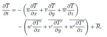
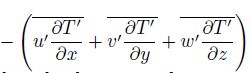 . The anomaly is defined as the deviation relative to the climatological monthly averaged value. As numerous studies have reported, NDH plays an important role in temperature asymmetry and its rectified effect on the mean state(Su et al., 2010; Cai and Qiu, 2013; Sun et al., 2014). Note that the long-term mean temperature trend approaches zero; moreover, if we ignore the residual term R, the long-term mean NDH and mean advection generally cancel each other. From the temperature equation, the mean temperature change is balanced by the dynamical terms mainly containing NDH and mean advection. This balance determines the structure of the mean temperature change. If there is a close spatial correlation between the temperature change and NDH/mean advection, it likely implies that NDH or mean advection favors the temperature change.
3. Model verification
. The anomaly is defined as the deviation relative to the climatological monthly averaged value. As numerous studies have reported, NDH plays an important role in temperature asymmetry and its rectified effect on the mean state(Su et al., 2010; Cai and Qiu, 2013; Sun et al., 2014). Note that the long-term mean temperature trend approaches zero; moreover, if we ignore the residual term R, the long-term mean NDH and mean advection generally cancel each other. From the temperature equation, the mean temperature change is balanced by the dynamical terms mainly containing NDH and mean advection. This balance determines the structure of the mean temperature change. If there is a close spatial correlation between the temperature change and NDH/mean advection, it likely implies that NDH or mean advection favors the temperature change.
3. Model verification
Forced with the observed wind stress and heat flux, the ocean model well captured the basic characteristics of the observed mean state. Figure 1 presents the climatological mean temperature and its annual st and ard deviation in the equatorial upper ocean(2°N–2°S)as a function of longitude and depth in the two basins, in which both the simulation and reanalyses were used from 1958 to 2001. These plots demonstrate that the model could capture the basic structure of the observed temperature, including the depth and tilt of the equatorial thermocline. In the Pacific, the model succeeds in describing the spatial pattern of the thermocline, which is deeper in the west and shallower in the east, and the large-scale pattern of the simulated temperature coincides well with the reanalysis; however, the simulated temperature near the western boundary is approximately 1℃ higher than that obtained from the reanalysis. Meanwhile, an excessive cold tongue and cold bias are shown in the equatorial eastern Pacific in WSA. In the Indian Ocean, the model also well reproduces the spatial structure of the observed thermocline, which is shallower in the western basin and deeper in the eastern basin. Both the observed and simulated tilts of the thermocline are opposite to those in the Pacific because the annual averaged wind stress prevailing in the equatorial Indian Ocean is westerly, but that in the Pacific is easterly. The simulated depth of the mean thermocline is almost 120 m, which agrees well with the reanalysis. However, there still exists some model bias; for instance, the simulated vertical temperature gradient is smaller than that obtained from the reanalysis. In general, the overall pattern simulated by LICOM2.0 resembles the reanalysis in the two basins(implying that the model has enough simulation ability), and a few discrepancies, such as cold bias in the equatorial eastern Pacific, are attributed to the coarse resolution of the model. The simulated st and ard deviation in the tropical Pacific agrees well with the reanalysis except for the smaller magnitude along the thermocline. In the Indian Ocean, the spatial pattern of the st and ard deviation is basically similar to the reanalysis, although there are differences in magnitude.

|
| Fig. 1 Temperature(℃; contour) and annual st and ard deviation(> 0.3 with color)in the equatorial upper Pacific and Indian Oceans(2°N–2°S)in(a, b)SODA,(c, d)WSA, and (e, f)the corresponding temperature(contour) and st and ard deviation(color)differences between WSA and SODA. |
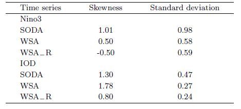
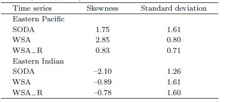
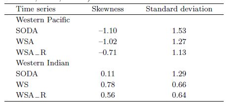
One of the principal causes of the simulated sea surface temperature anomalies as a response to the observed wind stress is ENSO in the tropical Pacific and IOD in the Indian Ocean. The observed ENSO/IOD variability was well reproduced by the OGCM, as shown in Fig. 2, which compares the time series of the Nino3/IOD index from the reanalysis with that from the WSA/WSA_R experiments. The simulated time series of the Nino3 from the WSA/WSA_R indices have correlations of 0.87/–0.79 with those from the reanalysis and 0.66/–0.50 for IOD index. The time series of the Nino3 from WSA has correlations of –0.92 and –0.72 with those from WSA_R and from the IOD index, respectively. The correlation between the time series of Nino3 and the IOD index is 0.36,0.29, and 0.27 for the reanalysis, WSA, and WSA_R, respectively. The simulated time series from WSA has a similar temporal evolution to that obtained from the reanalysis, but the simulated amplitude is weaker, especially for the IOD index. This discrepancy is expected, given that the thermal boundary conditions are simplified and that the SST is restored to the observed climatological datasets(Levitus and Boyer, 1994; Levitus et al., 1994). Moreover, because of the stronger magnitude associated with positive ENSO/IOD phases than with negative phases, the positive asymmetry can be found in both Nino3 and IOD indices(WSA experiment). More details can be seen in Table 1. Both the Nino3 and IOD indices show the temporal evolution at the surface, but the changes in the temperature anomalies in the subsurface also play an important role in ENSO/IOD dynamics. Therefore, the time series of the subsurface temperature anomalies in the eastern/western Pacific and Indian Ocean are presented for SODA, WSA, and WSA_R in Fig. 2. In addition, the skewness and st and ard deviation of subsurface temperature anomalies can be seen in Table 2 and Table 3.

|
| Fig. 2 (a, b)Nino3 and IOD index,(c, d)temperature anomalies in subsurface of eastern Pacific(2°N–2°S,100°W; 100 m) and eastern Indian Ocean(2°N–2°S,95 °E; 60 m), and (e, f)temperature anomalies in subsurface of western Pacific(2°N–2°S,160°W; 100 m) and western Indian Ocean(2°N–2 °S,45°E; 120 m)from SODA data(black line), WSA(red line), and WSA_R(green line). |
 |
 |
 |
It is well known that ENSO is the most important coupled ocean-atmosphere phenomenon in the tropical Pacific(Zebiak and Cane, 1987; Battisti,1988) and the first EOF mode of the equatorial subsurface temperature anomalies is ENSO(Cai et al., 2003; Rodger et al., 2004; Choi et al., 2013). Therefore, temperature asymmetry in the equatorial Pacific is mostly induced by ENSO asymmetry. Similarly,Cai et al.(2008)found, using temperature data from Scripps Institute of Oceanography, that the first EOF mode of the subsurface temperature anomalies is described by an eastwest dipole in the equatorial Indian Ocean. With SODA reanalysis data, we reached the same conclusion(figure omitted). In other words, the IOD mode is the first EOF mode for subsurface temperature anomalies, and the subsurface temperature asymmetry in the equatorial Indian Ocean also results from the IOD asymmetry. As suggested by An et al.(2005), skewness is an effective metric to quantify the asymmetry of temperature anomalies. Figure 3 illustrates temperature skewness as a function of longitude and depth in the upper equatorial ocean(2°N–2°S). The positive(negative)skewness implies that the strength of warm(cold)anomalies is larger than that of cold(warm)anomalies. The skewness from WSA coincides well with that of SODA in the upper ocean. The maximum positive skewness is at 100 m at around 100°W, and the largest negative skewness is at the same depth at around 160°E. However, the positive skewness occurs in the region(170°E–160°W; 0–80 m)that is different from SODA; and a small amount of negative skewness around 140°W in the upper 40 m in WSA is not found in SODA. Although there exist some discrepancies, the model could still represent the most significant skewness in the subsurface. In WSA_R, the location of the extreme center is not exactly the same as that in WSA, but there is a common phenomenon at a depth of 40–160 m. Meanwhile, the quantitative difference between the skewness from WSA and WSA_R is not negligible. From WSA minus WSA_R(figure omitted), we found that the largest positive value was 2.5 and was located at 100 m at around 100°W, while the largest negative value was –2 at 100 m at around 160°E. This result means that both the positive skewness in the equatorial eastern Pacific and the negative skewness in the western Pacific are stronger in WSA than in WSA_R.

|
| Fig. 3 Skewness of temperature in equatorial upper Pacific and Indian Oceans(2 ° N–2 ° S)in(a, b)SODA,(c, d)WSA, and (e, f)WSA_R. |
In the Indian Ocean, the skewness results from WSA and WSA_R and those from SODA are similar in the upper 140 m. There exists negative skewness in the upper 100 m of the equatorial eastern basin and positive skewness at 100–140 m. The largest negative skewness is between 90°–100°E at 20–40 m for both simulations and SODA, but the simulated values are larger. The positive skewness for WSA and WSA_R is also greater than that for SODA. The quantitative difference between the skewness results of WSA and WSA_R in the Indian Ocean(figure omitted)revealed that the largest negative skewness was nearly –7 and was located at 140 m between 80°–90°E, with a negative minimum of around –1 at 20–40 m between 90° and 100°E. Thus, considering the skewness difference between WSA and WSA_R, the negative skewness was slightly larger in the upper eastern Indian Ocean in WSA; more significant positive skewness was exhibited below 100 m in the eastern basin in WSA_R. The quantitative difference between WSA and WSA_R cannot be ignored in the two basins, which means that the asymmetry of the wind stress anomalies would cause changes in the magnitude of the temperature skewness. Specifically, the thermocline responses to the reversed wind stress anomalies were asymmetric. The thermocline became shallower when easterly wind stress anomalies occurred and deeper when westerly anomalies of the same magnitudes occurred. The more significant positive skewness in WSA_R is attributed to the stronger oceanic responses to the westerly wind stress anomalies. Furthermore, even if the climatological mean wind stress was applied in the control run, the simulated temperature still exhibited some skewness that was entirely different from that obtained from the reanalysis, WSA, and WSA_R(figure omitted). We found that the large-scale spatial pattern in the control run was obviously different from that in other plots, for example, differences in the location of the significant skewness and in the magnitude of the skewness. Considering the above findings, we conclude that the temperature skewness in the upper 40–160 m in the Pacific, and in the upper 140 m in the Indian Ocean, is not associated with the skewness of the wind stress. Our results resemble Figs. 6 and 7c in Ogata et al.(2013); the skewness was zero in numerical experiments with wind stress anomalies as the external forcing(Ogata et al., 2013), but the SST response was strongly negatively skewed. The numerical experimental design in our study was not identical to that of Ogata et al., but the conclusions are similar. Therefore, the temperature asymmetry in the subsurface to the first order may be attributed to the internal dynamical response to the external forcing.
4.1.2 Role of NDH in ENSO/IOD asymmetryBesides the skewness of the temperature anomalies, another metric to quantify asymmetry is the residual of temperature anomalies associated with positive and negative phases of ENSO/IOD events(Rodgers et al., 2004; Su et al., 2010; Ogata et al., 2013; Sun et al., 2014). We performed heat budget analysis in the positive and negative phases of ENSO/IOD events(figure omitted). The results showed that the zonal and meridional terms of NDH enhanced the positive temperature anomalies in the warm events in the upper equatorial eastern Pacific but weakened the negative anomalies in the cold events. The vertical term of NDH contributed greatly to temperature decrease in the warm events in the equatorial eastern Indian Ocean, but mitigated temperature increase in the cold events. Our findings based on the numerical experiments are consistent with those from reanalysis data by Su et al.(2010).
4.2 Heat budget in the mixed layerFigure 4 illustrates the temperature asymmetry in the mixed layer. In the Pacific, negative skewness exists in the southeastern basin(3°N–5°S,140°– 80°W)in WSA_R, but the opposite occurs in WSA. This difference indicates that the skewness of the wind stress anomalies would play a role in the skewness of the temperature anomalies in such a region. However, there is a common negative skewness in the western Pacific(120°–160°E) and in the southeastern tropical Indian Ocean, which confirms the more significant role of ocean dynamics in such regions.

|
| Fig. 4 As in Fig. 3, but for mixed layer condition. |
Because of asymmetry, the residual of the positive and negative phases of ENSO/IOD events is either much larger or smaller than zero. The spatial pattern of the residual of ENSO/IOD events is similar to that of the above temperature asymmetry. Given the fact that warm and cold temperature anomalies cannot completely cancel each other out, the long-term mean ENSO/IOD events should influence the climatological mean state or decadal oscillation, as has also been suggested by some recent studies(Rodger et al., 2004; Yu and Kim, 2011; Choi et al., 2012). As shown in Fig. 5, although the climatological mean wind stress used in all numerical experiments was identical, the simulated climatological mean temperature differs between the sensitivity experiments and control run. In the Pacific, due to interannual wind stress forcing, the simulated mean temperature in both WSA and WSA_R is 1℃ colder than that of the control run in the equatorial western Pacific, while the warm anomalies show a maximum of around 1℃ in the equatorial eastern Pacific. In the Indian Ocean, both WSA and WSA_R show temperature decreases in the upper 80 m in the equatorial eastern basin and temperature increases along the thermocline at 80–160 m in the Indian Ocean. In terms of the subsurface, the large-scale spatial pattern in Fig. 5 is similar to that of Fig. 3, but the locations of the maximum/minimum values in Fig. 5 are not exactly identical to those in Fig. 3. In Fig. 5, the time-mean effect from WSA has a high spatial correlation with WSA_R, implying that the mean temperature change in the subsurface is due to the asymmetry of the oceanic response to the anomalous surface forcing. Besides the temperature change, the current and salinity differences between the sensitivity experiments and control run showed identical behaviors(figure omitted). Furthermore, we conducted an additional experiment to confirm the above results. The experiment was designed to force the ocean model using idealized interannual wind stress anomalies but without any asymmetry. The time-mean temperature differences between the simulation results from this experiment and those from the control run were consistent with Fig. 5.

|
| Fig. 5 Temperature differences between control run and (a, c)WSA and (b, d)WSA_R in equatorial upper Pacific and Indian Oceans(2 ° N–2 ° S). |
Because the observed wind stress anomalies revealed obvious interannual variations, there existed dramatic interannual variations in the simulated temperatures and currents of the sensitivity experiments; however, these were negligible in the control run. Consequently, the climatological mean nonlinear advection terms in the sensitivity runs were different from those in the control run. Liang et al.(2012) and Sun et al.(2014)noted that ENSO rectification of the mean state is induced by the nonlinear heating terms of the heat budget formula. Therefore, we present NDH differences between the sensitivity runs(WSA and WSA_R) and the control run(Fig. 6), respectively. The results in the Figs. 6a and 6c are similar to those in Figs. 6b and 6d for the two basins, indicating that the situation is concurrent with Fig. 5. Only a minor difference between WSA and WSA_R can be found, in which the maximum difference is limited to 0.1 ℃ mon−1. In the Pacific, the largest positive NDH occurs at 20–60 m between 100° and 80°W, but the negative NDH mainly exists in the upper 80 m between 120° and 160°E. The warming center is located at 20–60 m between 100° and 80°W in Fig. 5, while the cooling center at 120 m is around 160°E. Thus, the mean temperature change in the equatorial eastern Pacific(Fig. 5)could be explained by NDH, but the temperature decrease in the equatorial western Pacific could not. In the Indian Ocean, the largest negative NDH is located at 20–80 m between 85° and 98°E, and the largest positive NDH is at 80– 120 m between 70° and 80°E. The cooling center is located at 20–80 m between 85° and 98°E in Fig. 5, and the warming center is at 80–120 m between 70° and 100°E. Therefore, NDH could explain the temperature decrease in the Indian Ocean, as well as in the partial warming region. To sum up, NDH favors the rectified effect of temperature asymmetry on the mean state. Further research(Hua et al., 2015)has shown that the upper ocean temperature and velocity anomalies(T′, u′, v′, w′)respond linearly to wind stress anomalies. Therefore, the significant correlation between the temperature anomaly(T′) and velocity anomalies(u′, v′, w′)( and thus the NDH)retains the same sign even though the wind stress anomalies are reversed. In this way, the impact of the rectification on the mean state remains almost unchanged.

|
| Fig. 6 Differences in NDH between control run and (a, c)WSA and (b, d)WSA_R in equatorial upper Pacific and Indian Oceans(2 ° N–2 ° S). |
We further compared the three components of the NDH with the total NDH(figure omitted) and found that the most important components were the zonal and meridional in the Pacific Ocean, while the key component was the vertical in the Indian Ocean.
5.1.3 Role of mean advection in ENSO/IOD rectificationGiven the fact that NDH could not account for the mean state change in some regions, such as the western Pacific,Fig. 7 shows the differences in mean advection between the sensitivity runs(WSA and WSA_R) and control run. In the Pacific, the cold advection corresponding with the cold temperature anomalies covers the western region(140°E–160°W)below 100 m. The warm advection is located at 0–20 m between 120° and 80°W, and it is also in line with the warm anomalies near the surface of the Pacific in Fig. 5. In the Indian Ocean, the warm advection center is located at 60–120 m between 90° and 100°E, which could well explain the warm anomalies near the eastern boundary of the Indian Ocean in Fig. 5. The cold advection below 120 m covers the partial region with cold anomalies in Fig. 5. Considering that neither the total NDH nor the mean advection could provide an adequate explanation of the mean state change, the non-linearity of the vertical mixing(R in the temperature formula)should also play a role. The largest temperature differences mainly occurred around the thermocline, where vertical mixing cannot be ignored. Moreover, because any vertical mixing scheme is nonlinear and dependent on the mean state, it is vital to diagnose the contribution of vertical mixing to the heat budget in future studies. Although temperature change is related, to some extent, to vertical mixing, underst and ing the effects of NDH and mean advection on the mean state is essential.

|
| Fig. 7 Differences in mean advection between control run and (a, c)WSA and (b, d)WSA R in equatorial upper Pacific and Indian Oceans(2 ° N–2 ° S). |
The pattern of mean temperature change in the mixed layer from WSA_R(Fig. 8), illustrating the importance of nonlinear dynamics. As can be seen, the temperature increases in the eastern Pacific(15°S–10°N,120°–80°W) and decreases in the western Pacific(140°–160°E). In the Indian Ocean, there is a warming center located over 0°–10°S,40°–80°E, and there are also some cooling regions such as north of equator, south of 10°S.

|
| Fig. 8 As in Fig. 5, but for mixed layer condition. |
Figure 9 further shows the corresponding differences in the NDH between the sensitivity runs and control run. The NDH contributes much to the cooling region in the western Pacific(140°–160°E)as well as to some warming regions(0°–3°N,120°–80°W). In the Indian Ocean, the NDH shows a negative value in most regions that cover the cooling regions in Fig. 8.

|
| Fig. 9 As in Fig. 6, but for most important components, i.e.,(a, b)zonal NDH for Pacific and (c, d)vertical NDH for Indian Ocean, in mixed layer condition. Units are ℃ month −1 |
The mean advection differences are shown in Fig. 10. These can explain the temperature increases in most regions of the eastern Pacific(15°S–15°N,120°– 80°W) and also the warming center(0°–10°S,40°– 80°E)in the Indian Ocean.

|
| Fig. 10 As in Fig. 7, but for most important components, i.e., vertical advection for(a, b)Pacific and (c, d)Indian Oceans, in mixed layer condition. Units are ℃ month −1. |
The temperature anomalies associated with ENSO/IOD in the tropical Pacific and Indian Oceans not only show significant asymmetry, but also have a rectification effect on the mean state or decadal climate variations. We conducted several numerical experiments with an OGCM in this study. These experiments were designed(1)to evaluate the model’s ability to reproduce the interannual variations, especially the temperature asymmetry in tropical basins;(2)to help quantify the relative contributions of wind stress forcing and ocean dynamical processes to the asymmetry of temperature anomalies; and (3)to underst and the rectification effect of the interannual variations on the mean state and its physical mechanism.
When forced by the observed wind stress with interannual anomalies, the model well reproduced the large-scale patterns of the mean states in these two basins. Meanwhile, the general spatial pattern of temperature asymmetry simulated by the ocean model was similar to the reanalysis in the upper 40–160 m in Pacific and 0–140 m in Indian Ocean. The asymmetry in such subsurface regions mainly results from the nonlinear response to the surface wind stress anomalies through internal dynamic processes, rather than the skewness of winds. The climatological mean states simulated by the two numerical experiments were alike, but different from that of the control run, which indicates that the two sensitivity runs, in which the wind stress anomalies were opposite to each other, exerted similar time-mean effects on the mean state. Further analysis showed that NDH plays a crucial role in the warming of the equatorial eastern Pacific below 20 m and in the cooling of the upper equatorial eastern Indian Ocean. Mean advection contributes much to the cooling in the equatorial western Pacific below 100 m as well as to the warming at the eastern boundary of the Indian Ocean.
There are some interannual variation modes in SST anomalies in the tropical Atlantic(Servain,1991; M´elice and Servain, 2003), but previous studies have rarely addressed the temperature asymmetry in this basin. Besides numerical experiments in the Pacific and Indian oceans, we conducted similar numerical experiments in the tropical Atlantic(30°N–30°S,80°W– 20°E)in this study. Comparison of these simulations indicated that the asymmetric responses of the temperature and velocity anomalies to the wind stress anomaly are highly universal in the tropical oceans; temperature anomalies are less asymmetric in the tropical Atlantic than they are in the tropical Pacific NO.4 HUA Lijuan and YU Yongqiang 625 and Indian oceans, and the corresponding rectification of the mean state is also much weaker.
| An, S. I., and Jin Feifei, 2001: Collective role of thermocline and zonal advective feedbacks in the ENSO mode. J. Climate, 14, 3421-3432. |
| An, S. I., and Jin Feifei, 2004: Nonlinearity and asymmetry of ENSO. J. Climate, 17, 2399-2412. |
| An, S. I., Y. G. Ham, J. S. Kug, et al., 2005: El Niño-La Niña asymmetry in the coupled model intercompar-ison project simulations. J. Climate, 18, 2617-2627. |
| Battisti, D. S., 1988: Dynamics and thermodynamics of a warming event in a coupled tropical atmosphere-ocean model. J. Atmos. Sci., 45, 2889-2919. |
| Burgers, G., and D. B. Stephenson, 1999: The “normality” of El Niño. Geophys. Res. Lett., 26, 1027-1030, doi: 10.1029/1999GL900161. |
| Cai Wenju, H. H. Hendon, and G. Meyers, 2005: Indian Ocean dipolelike variability in the CSIRO Mark 3 coupled climate model. J. Climate, 18, 1449-1468. |
| Cai Wenju and Qiu Yun, 2013: An observation-based assessment of nonlinear feedback processes associ-ated with the Indian Ocean dipole. J. Climate, 26, 2880-2890. |
| Cai Yi, Wang Zhanggui, Yu Zhouwen, et al., 2003: The EOF analysis of temperature and zonal flow in the equatorial Pacific Ocean and the study of the El Niño forecasting. Acta Oceanol. Sinica, 25, 12-18. (in Chinese) |
| Cai Yi, Li Hai, and Zhang Renhe, 2008: A study on the relationship between ENSO and tropical Indian Ocean temperature. Acta Meteor. Sinica, 66, 120-124. (in Chinese) |
| Canuto, V. M., and M. S. Dubovikov, 2005: Modeling mesoscale eddies. Ocean Modeling, 8, 1-30. |
| Carton, J. A., and B. S. Giese, 2008: A reanalysis of ocean climate using simple ocean data assimilation (SODA). Mon. Wea. Rev., 136, 2999-3017. |
| Choi, J., S. I. An, and S. W. Yeh, 2012: Decadal amplitude modulation of two types of ENSO and its relationship with the mean state. Climate Dyn., 38, 2631-2644. |
| Choi, J., S. I. An, S. W. Yeh, et al., 2013: ENSO-like and ENSO-induced tropical Pacific decadal variability in CGCMs. J. Climate, 26, 1485-1501. |
| Fedorov, A. V., and S. G. Philander, 2001: A stability analysis of tropical ocean-atmosphere interactions: Bridging measurements and theory for El Niño. J. Climate, 14, 3086-3101. |
| Gent, P. R., and J. C. McWilliams, 1990: Isopycnal mix-ing in ocean circulation models. J. Phys. Oceanogr., 20, 150-155. |
| Hua Lijuan, Yu Yongqiang, and Yin Baoshu, 2010: Nu-merical modeling of the asymmetry of Indian Ocean dipole and its mechanism. Chinese J. Atmos. Sci., 34, 1046-1058. (in Chinese) |
| Hua Lijuan, Yu Yongqiang, and Sun Dezheng, 2015: A further study of ENSO rectification: Results from an OGCM with a seasonal cycle. J. Climate, 28, 1362-1382. |
| Hong, C. C., T. Li, L. Ho, et al., 2008: Asymmetry of the Indian Ocean dipole. Part I: Observational analysis. J. Climate, 21, 4834-4848. |
| Large, W. G., G. Danabasoglu, S. C. Doney, et al., 1997: Sensitivity to surface forcing and boundary layer mixing in a Global Ocean Model: Annual-mean cli-matology. J. Phys. Oceanogr., 27, 2418-2447. |
| Levitus, S., and T. P. Boyer, 1994: World Ocean Atlas 1994 Volume 4: Temperature. NOAA Atlas NES-DIS 4. US Department of Commerce, Washington D.C., 1-117. |
| Levitus, S., R. Burgett, and T. P. Boyer, 1994: World Ocean Atlas 1994 Volume 3: Salinity. NOAA Atlas NESDIS 3. US Department of Commerce, Washing-ton D.C., 1-99. |
| Li Yangchun, Xu Yongfu, Chu Min, et al., 2012: Influ-ences of climate change on the uptake and storage of anthropogenic CO2 in the global ocean. Acta Meteor. Sinica, 26, 304-317, doi: 10.1007/s13351-012-0304-z. |
| Liang Jin, Yang Xiuqun, and Sun Dezheng, 2012: The effect of ENSO events on the tropical Pacific mean climate: Insights from an analytical model. J. Climate, 25, 7590-7606. |
| Liu Hailong, Zhang Xuehong, Yu Yongqiang, et al., 2004a: Manual for LASG/IAP Climate System Ocean Model. Science Press, Beijing, 1-108. (in Chinese) |
| Liu Hailong, Zhang Xuehong, Li Wei, et al., 2004b: An eddy-permitting oceanic general circulation model and its preliminary evaluation. Adv. Atmos. Sci., 21, 675-690. |
| Liu Hailong, Lin Pengfei, Yu Yongqiang, et al., 2012: The baseline evaluation of LASG/IAP Climate Sys-tem Ocean Model (LICOM) Version 2. Acta Meteor. Sinica, 26, 318-329, doi: 10.1007/s13351-012-0305-y. |
| Mélice, J. L., and J. Servain, 2003: The tropical Atlantic meridional SST gradient index and its relationships with the SOI, NAO, and southern Ocean. Climate Dyn., 20, 447-464. |
| Ogata, T., Xie Shangping, Lan Jian, et al., 2013: Im-portance of ocean dynamics for the skewness of the Indian Ocean dipole mode. J. Climate, 26, 2145-2159. |
| Ohba, M., and H. Ueda, 2009: Role of nonlinear atmo-spheric response to SST on the asymmetric transi-tion process of ENSO. J. Climate, 22, 177-192. |
| Okumura, Y. M., and C. Deser, 2010: Asymmetry in the duration of El Niño and La Niña. J. Climate, 23, 5826-5843. |
| Rodgers, K. B., P. Friederichs, and M. Latif, 2004: Trop-ical Pacific decadal variability and its relation to decadal modulations of ENSO. J. Climate, 17, 3761-3774. |
| Roeske, F., 2001: An Atlas of Surface Flues Based on the ECMWF Reanalysis-A Climatological Dataset to Force Global Ocean General Circulation Models. Report No. 23, Hamburg: Max-Planck-Institut für Meteorologie, 1-31. |
| Rong Xinyao, Zhang Renhe, T. Li, et al., 2011: Upscale feedback of high-frequency winds to ENSO. Quart. J. R. Meteor. Soc., 137, 894-907. |
| Saji, N. H., B. N. Goswami, P. N. Vinayachandran, et al., 1999: A dipole mode in the tropical Indian Ocean. Nature, 401, 360-363. |
| Saji, N. H., and T. Yamagata, 2003: Structure of SST and surface wind variability during Indian Ocean dipole mode events: COADS observations. J. Climate, 16, 2735-2751. |
| Servain, J., 1991: Simple climatic indices for the tropical Atlantic Ocean and some applications. J. Geophys. Res., 96, 15137-15146. |
| Su Jingzhi, Zhang Renhe, T. Li, et al., 2010: Causes of the El Niño and La Niña amplitude asymmetry in the equatorial eastern Pacific. J. Climate, 23, 605-617. |
| Sun Dezheng, 2003: A possible effect of an increase in the warm-pool SST on the magnitude of El Niño warming. J. Climate, 16, 185-205. |
| Sun Dezheng and Zhang Tao, 2006: A regulatory effect of ENSO on the time-mean thermal stratification of the equatorial upper ocean. Geophys. Res. Lett., 33, L07710. |
| Sun Dezheng, Zhang Tao, Sun Yan, et al., 2014: Rectifi-cation of El Niño-Southern Oscillation into climate anomalies of decadal and longer time scales: Results from forced ocean GCM experiments. J. Climate, 27, 2545-2561. |
| Sun Yan, Sun Dezheng, Wu Lixin, et al., 2012: The western Pacific warm pool and ENSO asymmetry in CMIP3 models. Adv. Atmos. Sci., 30, 940-953. |
| Uppala, S. M., P. W. Kållberg, A. J. Simmons, et al., 2005: The ERA-40 re-analysis. Quart. J. Roy. Me-teor. Soc., 131, 2961-3012. |
| Yan Bangliang and Zhang Renhe, 2002: The role of at-mosphere climate basic state in the formation of westerly over the equatorial Pacific. Acta Oceanol. Sin., 24, 39-50. (in Chinese) |
| Yu Jinyi and S. T. Kim, 2011: Reversed spatial asymme-tries between El Niño and La Niña and their linkage to decadal ENSO modulation in CMIP3 models. J. Climate, 24, 5423-5434. |
| Yu Yongqiang, Zheng Weipeng, Wang Bin, et al., 2011: Versions g1. 0 and g1.1 of the LASG/IAP flexible global ocean-atmosphere-land system model. Adv. Atmos. Sci., 28, 99-117. |
| Zebiak, S. E., and M. A. Cane, 1987: A model El Niño-Southern oscillation. Mon. Wea. Rev., 115, 2262-2278. |
| Zhang Tao, Sun Dezheng, R. Neale, et al., 2009: An evaluation of ENSO asymmetry in the community climate system models: A view from the subsurface. J. Climate, 22, 5933-5961. |
| Zheng Xiaotong, Xie Shangping, G. A. Vecchi, et al., 2010: Indian Ocean dipole response to global warm-ing: Analysis of ocean-atmospheric feedbacks in a coupled model. J. Climate, 23, 1240-1253. |
| Zhong Aihong, H. H. Hendon, and O. Alves, 2005: Indian Ocean variability and its association with ENSO in a global coupled model. J. Climate, 18, 3634-3649. |