 2015, Vol. 28
The Chinese Meteorological Society
Article Information
- WANG Yongdi, JIANG Zhihong, CHEN Weilin. 2015.
- Performance of CMIP5 Models in the Simulation of Climate Characteristics of Synoptic Patterns over East Asia
- J. Meteor. Res., 28(4): 594-607
- http://dx.doi.org/10.1007/s13351-015-4129-4
Article History
- Received 2014-12-30;
- in final form 2015-05-25


2 School of Geography and Remote Sensing, Nanjing University of Information Science & Technology, Nanjing 210044
Global climate models (GCMs) are a useful tool for simulating the present climate and for projecting the future climate. Evaluating the ability of climate models in simulating various features of large-scale circulations is essential for providing useful information upon selecting appropriate GCMs for research of future climate prediction and downscaling.
Using the outputs of the Coupled Model Intercomparison Project Phase 3 (CMIP3), researchers have evaluated the ability of GCMs in simulating circulations over East Asia (Zhou et al., 2009; Zhou and Zou, 2010; Li et al., 2011a,b; Zhou and Zhang, 2011). Previous studies show that the CMIP3 models have some ability in regional climate simulation over East Asia (Zhou and Yu, 2006; Liu and Jiang, 2009). Large differences, however, existed among different GCMs. The models’ ability in simulating the East Asian monsoon was weak overall (Zhao et al., 2013). For example, large model biases existed in the Qinghai-Tibetan Plateau area (Zhang and Chen, 2011; Bao et al., 2014), and the simulations of the western Pacific subtropical high and the Mongolian high were poor (Guo et al., 2012; Liu et al., 2014). Recently, several studies on the Coupled Model Intercomparison Project Phase 5 (CMIP5) model simulations over East Asia were performed (Xu and Xu, 2012a,b; Zhang,2012; Chen,2013; Sperber et al., 2013; Song and Zhou, 2014a,b; Song et al., 2014; He and Zhou, 2014,2015; Li et al., 2015). Jiang and Tian (2013) assessed the simulations of the climate conditions during the winter and summer monsoons over East Asia. They concluded that the overall strength of the East Asian winter monsoon did not have any trend when considered against the background of global warming. Simulation of the western Pacific subtropical high was evaluated by Liu et al. (2014). They concluded that most models showed a strong ability in simulating spatial patterns and amplitudes of the geopotential height field and zonal wind changes. Sperber et al. (2013) found that, in terms of the multi-model mean, the CMIP5 models outperformed the CMIP3 models in all of the diagnostics. Song and Zhou (2014a) reported that the CMIP5 multimodel ensemble mean showed a significant improvement over CMIP3 for the interannual East Asian summer monsoon (EASM) pattern.
Many studies have evaluated the climatological monthly-mean state of circulations, annual variation, and interannual and interdecadal variability of circulation patterns. In many cases, however, it is also necessary to evaluate synoptic patterns and their frequency distribution on daily timescales. In recent years, studies of extreme weather events against the background of global climate change have attracted increasing attention. A strong link exists between changes in extreme weather events and changes in synoptic patterns in terms of variation in both intensity and frequency (Dayan et al., 2012; Paraschivescu et al., 2012; Raziei et al., 2012; Cohen et al., 2013). This means that the climate characteristics of synoptic-scale cyclone activity (such as frequency, intensity, and duration) are closely linked to those of extreme weather events. However, according to Liu et al. (2006a, b), Liu and Weisberg (2005), and Reusch et al. (2005, 2007), model evaluation of the climate characteristics for synoptic-scale patterns (referred to as circulation patterns or CP hereafter) using traditional statistical methods (such as empirical orthogonal function or principal component analysis (PCA) and statistical indicators) is less accurate and less intuitive. Recently, Radić and Clarke (2011) used self-organizing maps (SOMs), an advanced nonlinear data analysis method, to evaluate Intergovernmental Panel on Climate Change Fourth Assessment Report (IPCC AR4) models in terms of their ability in simulating the CP over North America. A multitude of characteristic synoptic patterns and their occurrence frequencies within the study area were acquired. Model ability in simulating the synoptic-scale CP was evaluated quantitatively by calculating the correlation coefficient between the frequencies of modeled patterns and frequencies of NCEP reanalysis patterns. Their research suggested that the SOM method was an effective tool to study a model’s ability in simulating synoptic patterns and their features. To our knowledge, there is less research on model evaluations of synoptic-scale weather features over the East Asia.
The SOM was proposed by Kohonen (1982), and was used in the study of atmospheric phenomenon by Hewitson and Crane (2002). After the variability in multi-dimensional meteorological datasets has gone through self-learning, and been trained and clustered according to the neural network principle, numerous characteristic synoptic patterns (e.g., winning neuron) and their evolution can be obtained (Reusch et al., 2007; Ning et al., 2012). This method has more advantages than PCA in distinguishing actual atmospheric synoptic patterns and their evolution (Reusch et al., 2005; Liu et al., 2006a,b). At present, SOM has been used in climate diagnosis, model evaluation, statistical downscaling, etc. The SOM method was used to examine the relationship between the local daily rainfall and humidity fields of large-scale circulation in northeastern and southeastern Mexico (Cavazos,2000). Daily synoptic patterns were extracted from sea level pressure (SLP) fields and assessed in terms of the ability of GCM models in simulating atmospheric circulation 596 JOURNAL OF METEOROLOGICAL RESEARCH VOL.29 patterns by SOMs (Finnis et al., 2009). Using SOMs,Schuenemann and Cassano (2009) classified the synoptic patterns in the North Atlantic region from 1961 to 1999. Detailed studies of the differences in various patterns between model output and observational data, including corresponding precipitation, were also performed (Schuenemann and Cassano, 2009). The deviations in annual precipitation simulation by 15 IPCC AR4 models were analyzed and attributed to differences in intra-pattern variability, differences in pattern frequency, and differences in pattern frequency acting on intra-pattern variability. These results showed that SOMs could be used as an effective tool to analyze the possible causes of differences between simulation and observation.
The simulation results of more than 50 models are available from the CMIP5 archives. Compared with the CMIP3 models, most CMIP5 models have been significantly improved in terms of model structure, resolution, physical processes, etc. (Taylor et al., 2012; Zhou et al., 2014). However, traditional statistical methods are inefficient in assessing of the climatic characteristics of daily circulation patterns. Therefore, it is important to assess the simulation ability of CMIP5 models in terms of the climate characteristics of daily CPs over East Asia. In this study, we use the SOM-based methodology introduced by Radić and Clarke (2011) to obtain the main synoptic patterns in daily SLP and their occurrence frequencies in both summer and winter. By comparing the similarity of characteristic synoptic pattern frequency distribution in the GCMs and NCEP, we evaluate how well the CMIP5 models reproduce the observed synoptic-scale atmospheric circulations over East Asia.
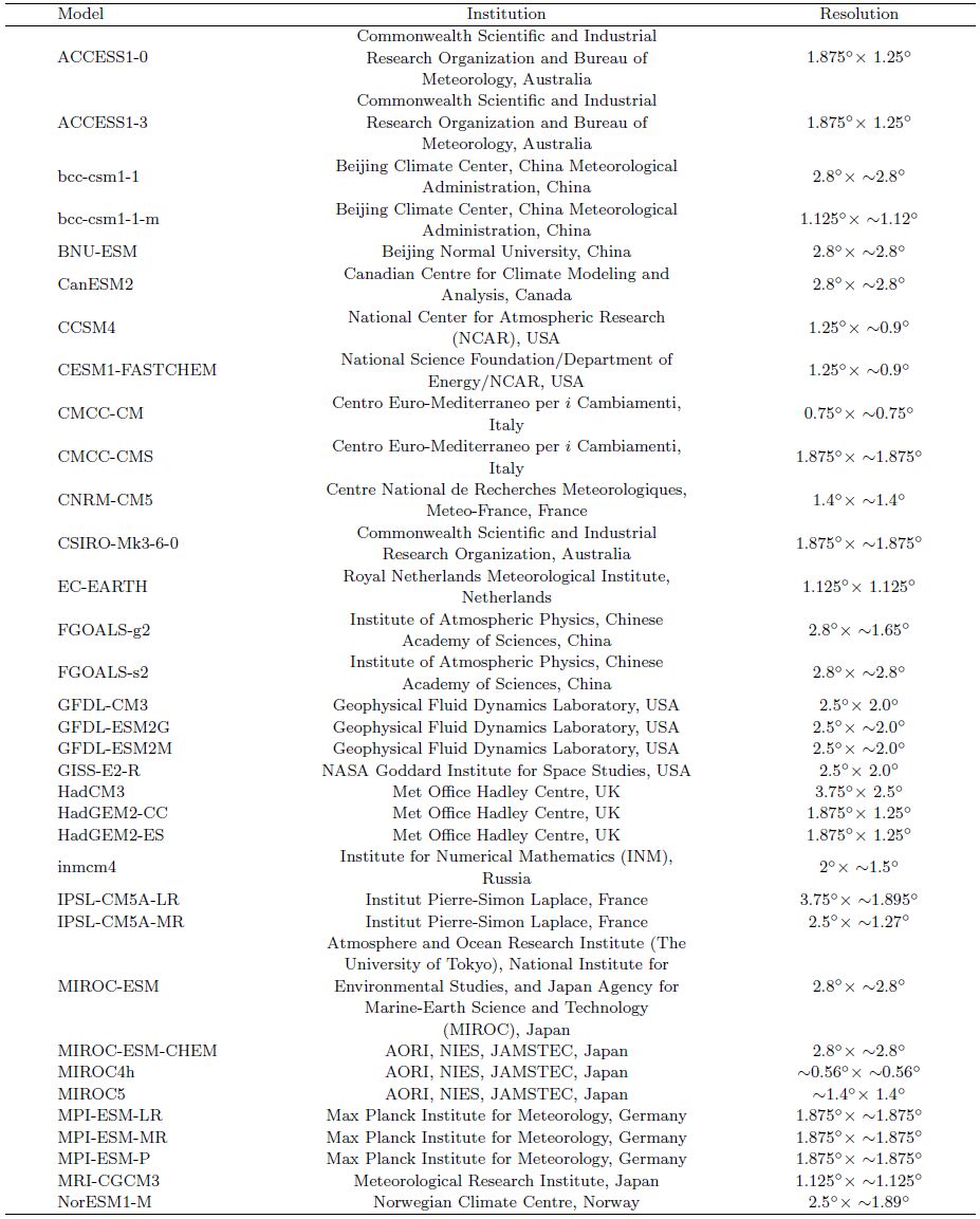
2. DataOur evaluation focuses on the 20-yr datasets of CMIP5 outputs during 1980-1999, which are based on the simulations (Run r1i1p1 of the “historical” simulation of CMIP5 models) by 34 GCMs (archived by the PCMDI at http://pcmdi9.llnl.gov/esgf-web-fe/). These models are listed in Table 1. To represent the synoptic patterns, we use the daily SLP field as the input data of the SOM training process.
 |
We compare GCM outputs with the NCAR/ NCEP reanalysis data (Kalnay et al., 1996), which are available from 1948 to the present. We assume that the NCAR/NCEP reanalysis is a reasonable proxy of the observation. To facilitate GCM intercomparison and validation against the NCAR/NCEP reanalysis, all model simulation outputs were interpolated to a common grid (with a resolution of 2.5°) by using bilinear interpolation. East Asia defined in this study is from 0° to 80°N, and from 20° to 180°E. Note that the SLP field over the Qinghai-Tibetan Plateau (25°- 40°N,74°-104°E) is not included in the analysis, because the model result there is not realistic.
3. Method 3.1 Brief description of SOMThe SOM is an unsupervised, artificial neural network based on competitive learning (Kohonen, 1982,2001). Characteristic synoptic patterns represent the nonlinear phases of the synoptic-scale circulation by self-learning and repeated competition. The SOM consists of two layers: input and competitive (output). Training and mapping are the two main processes in SOM training. In this study, the daily SLP field is used as the input layer of the SOM, and certain types of synoptic circulation mode are found as winning nodes (known as nodes) in the output layer. Each category is referred to as a node, and the number of nodes is specified by the user.
The general SOM training algorithm is summarized as follows:
(i) Establishment of the SOM network and its initialization. The SOM begins with a user-defined map size, and the number of circulation types is determined as needed. In order to represent the input data, the nodes of an SOM are first initialized (known as reference vectors). The SOM training proceeds by each reference vector learning iteratively from the input data. Then, a r and om weight vector is assigned to each node.
(ii) Calculation of the Euclidean distance (EUD) between the weight of each node’s reference vector and an input vector. This finds the minimum EUD between the weight vector of the jth node and the input data. EUD is defined as
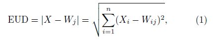
(iii) Finding the winning node. The EUD between the input sample and each node in the competitive (output) layer is calculated, and the node that is closest (having the smallest EUD) to the input vector is known as the winning node.
(iv) Updating the weight of each node. The node positions that are in the neighborhood of the winning neuron are updated. They are moved to the position that is closer to the input vector. Each node learns from the input data and shifts its position accordingly. Then, the SOM becomes topologically organized depending on the smallest EUD, resulting in similar nodes being adjacent to each other. Updating of the weight vector can be described as

(v) Updating the learning rate and neighborhood size. The next input vector is entered and steps (ii)-(v) are repeated.
(vi) Determining the termination condition. Training is interrupted when the number of iterations reaches the preset condition. The final winning node is the characteristic synoptic pattern extracted by the SOM.
Details of the SOM method can be found in Kohonen (2001) and Chu et al. (2012).
The choice of SOM node size is actually determined by the number of major synoptic patterns. In mathematics, the size of SOM nodes is determined in accordance with a principle: maximizing similarity within clusters and minimizing similarity between clusters. In this study, we use several different SOM sizes (the numbers of nodes being 3 × 3,4 × 4,5 × 5, and 6 × 6) to compare the training results. Relevant discussion and analysis are provided in Section 4.4.
3.2 Data preprocessingIn order to evaluate the ability of these models in terms of simulating daily synoptic patterns and their evolution, two types of anomalies are considered in our SOM analysis:
(1) The daily-averaged SLP over the 20-yr baseline period (1980-1999) is subtracted from the daily SLP at each grid point (for the NCEP reanalysis and for each GCM output). The resulting anomaly fields are employed in the SOM training. These temporal SLP anomalies are herein referred to as temporal SLP.
(2) For daily data, the average of each grid point within the study area is subtracted from the daily SLP at each grid point. The resulting anomaly fields are used for training. These spatial SLP anomalies are herein referred to as spatial SLP.
3.3 Evaluation of CMIP5 modelsAfter temporal and spatial SLP trainings in winter and summer, respectively, we obtain two kinds of SOM patterns in winter and summer. The simulation ability of each model can be assessed by comparing the frequencies of modeled patterns with the frequencies of observations. A good model can often reproduce the actual atmospheric synoptic patterns (here represented by the NCEP reanalysis data), and each weather pattern should have the same occurrence of frequency as that of the NCEP reanalysis. Therefore, a model’s simulation ability can be measured by the correlation coefficient between the frequencies of modeled patterns and frequencies of NCEP reanalysis patterns. A ranking of model simulation ability in terms of weather pattern characteristics can be obtained by using these coefficients.
4. Results and analysis 4.1 Synoptic patterns in observations4.1.1 Characteristic synoptic patterns of SOM in temporal SLP
Following Radić and Clarke (2011), using temporal SLP anomalies from the NCEP reanalysis, we obtained the synoptic patterns (with a map size of 4 × 4) of temporal SLP and analyzed their evolution characteristics in winter and summer for the period of 1980-1999. Figures 1a and 1b illustrate the characteristic daily SLP anomaly patterns in winter and summer, respectively, for this period over East Asia. The temporal SLP, with the daily-averaged SLP over the 20-yr baseline period (1980-1999) subtracted, reflects the daily evolution of major weather systems over East Asia because it indicates the daily anomalies in the reference period.
For winter, the most striking feature in the SOM pattern is the evolution of the Mongolian high, which is the dominant system of the East Asian winter monsoon. As shown in Fig. 1a, there is initially a notable positive anomaly in node (1,1). From nodes (1,1) to (1,4) (top panel), this positive anomaly becomes gradually weaker and moves eastward, accompanied by a negative anomaly appearing over the western region. From nodes (1,1) to (4,1) (left column) the positive anomalies move westward; at the same time, a negative anomaly emerges in the northeastern region. The above negative anomaly becomes stronger from nodes (1,4) and (4,1) to node (4,4). In other words, a cycle of one SOM pattern represents the evolution of the Mongolian high from a positive anomaly to a negative anomaly.

|
| Fig. 1 The 4 × 4 SOM patterns (hPa) in temporal SLP based on the 1980-1999 NCEP reanalysis data in (a) winter and (b) summer. |
During the summer months, the situation is more complicated than that in winter. Although the Mongolian high still exists, its magnitude change is much smaller than in winter, and its range of effect is mainly in high latitudes. In middle and lower latitudes, the Indian low-pressure system dwells. Meanwhile, there are some intensity changes of the subtropical high pressure system in the western Pacific. Therefore, the SOM patterns in Fig. 1b comprehensively reflect the major systems of the summer SLP. The characteristic anomalous changes of some systems can be identified, such as the Mongolian high in high latitudes, and the Indian low and West Pacific subtropical high in middle and lower latitudes.
4.1.2 Characteristic synoptic patterns of SOM in spatial SLPSince spatial SLP is based on the domainaveraged daily SLP and it focuses on spatial variability, it reflects the spatial pattern of major weather systems in the area. Figure 2a depicts the evolution of winter SLP based on the spatial SOM analysis. It can be seen that the Mongolian high is still the most important high pressure system. From nodes (1,1) to (4,4), an obvious variation process of the major pressure system position can also be seen. For example, nodes (1,1) → (4,1) → (4,4) and (1,1) → (1,4) → (4,4) show the process of the Mongolian high moving southward from the east and west sides, respectively.

|
| Fig. 2 The 4 × 4 SOM patterns (hPa) in spatial SLP based on the 1980-1999 NCEP reanalysis data in (a) winter and (b) summer. |
In the process from nodes (1,1) to (4,4), two opposite changes are seen in the Aleutian low and Icel and ic low pressure systems. The Icel and ic low pressure system enhances and exp and s gradually, and is accompanied by the Aleutian low system waning slightly. The change process of the summer major climate system is shown in Fig. 2b. Evolutions of the West Pacific subtropical high and Indian low pressures are clear. The nodes from (1,1) to (4,4) show that the subtropical high gradually exp and s and strengthens from east to west. In this process, the Indian low does not show any significant changes.
4.2 Performance of CMIP5 models in terms of occurrence frequency of synoptic patternsAfter creating the SOM classifications, the model performance could be evaluated. A model that can show similar synoptic patterns and similar frequencies of these patterns, to the NCEP reanalysis will be regarded as a good model. The node frequency (%) for a certain pattern was calculated as the total number of days of that pattern (node) divided by the total number of days in that season over the 20-yr baseline period. According to Radić and Clarke (2011), the success of a model depends on how well these frequencies from the model simulations correlate with the frequencies derived from the NCEP reanalysis. In order to determine the simulation ability of the synoptic patterns and frequencies of various CMIP5 models, an assessment was performed as follows.
(i) Each GCM is classified according to the SOM trained by the NCEP reanalysis to obtain the occurrence frequencies.
(ii) The frequencies of modeled patterns and those of the NCEP reanalysis patterns are compared, and the correlation coefficient between them is calculated. Thus, the simulation ability of these patterns and their frequencies in the SLP field can be assessed quantitatively.
We use the model of National Climate Center of China, bcc-csm1-1-m, as an example to describe the assessment results using the SOM method.
Figure 3 plots the frequency of each node from the NCEP reanalysis and bcc-csm1-1-m. The nodes in Figs. 3a and 3b correspond to the nodes in Figs. 1a and 1b, respectively. In the patterns of temporal SLP anomalies, a significant positive correlation (at the 95% confidence level) is obtained between the two seasons (winter: r = 0.66; summer: r = 0.90). A high positive correlation indicates that, for a given season over the baseline period, each pattern occurs in bcccsm1-1-m as often as in the NCEP reanalysis.

|
| Fig. 3 Comparison of the 4 × 4 SOM pattern frequencies of the NCEP reanalysis with those of bcc-csm1-1-m in temporal SLP in (a) winter and (b) summer. |
In the patterns of spatial SLP anomalies (Figs. 4a and 4b) the correlation is also significantly positive (winter: r = 0.63; summer: r = 0.73). This indicates that the simulation ability of bcc-csm1-1-m in spatial SLP is slightly weaker than that in temporal SLP. However, the occurrence of SLP spatial patterns in bcc-csm1-1-m is almost equal to their occurrence in the NCEP reanalysis. In other words, spatial SLP patterns that occur frequently in the NCEP reanalysis also occur frequently in bcc-csm1-1-m. We conclude that this model is able to capture occurrence frequencies of various SOM patterns in East Asia.

|
| Fig. 4 As in Fig. 3, but for spatial SLP. |
The temporal SLP and spatial SLP of the other CMIP5 models can also be projected onto the SOM nodes that are trained by using the NCEP reanalysis data in winter and summer, respectively. Correlation analysis was performed between the NCEP reanalysis and each of the 34 GCMs, for both temporal and spatial SLPs. The results for the temporal and spatial 4 × 4 SOMs over the study region are shown in Fig. 5. A correlation greater than 0.5 (at the 95% confidence level) is defined as significant.

|
| Fig. 5 Scatter plots of simulation frequency and NCEP reanalysis frequency in temporal and spatial SLP in (a) winter and (b) summer. |
For temporal SLP anomaly patterns (Fig. 5), many GCMs have significant positive correlations (r > 0.5) with the NCEP reanalysis in both winter and summer; specifically, the percentage in winter is 66.7% (23 out of 34) and in summer is 88.2% (30 out of 34). According to the high percentage of the significant positive correlations, we conclude that the frequencies of temporal SLP anomaly patterns in the NCEP reanalysis over the baseline period can be reproduced by most GCMs, and these models’ simulation ability is better in summer than in winter.
Most of the CMIP5 GCMs can simulate fairly well the frequencies of temporal SLP anomaly patterns, but analysis of spatial SLP anomaly patterns shows less encouraging results. The y-axis of Fig. 5 indicates that the percentage of significant positive correlations in winter is 20.6% (7 out of 34), while it is only 17.6% (6 out of 34) in summer. The small percentage of significant positive correlations means that very few CMIP5 models are able to reproduce the frequencies of spatial SLP anomaly patterns in the NCEP reanalysis in both winter and summer over the baseline period.
Based on these results of both temporal and spatial SLP, we conclude that most of the CMIP5 models have strong simulation ability in reproducing temporal SLP, but are poor in terms of spatial SLP. Our results in this study over East Asia are consistent with those in North America (Radić and Clarke, 2011).
4.3 Comparison of model ability in producing temporal and spatial SLPTo further investigate these differences in simulation ability, the contrast between model frequency and NCEP reanalysis frequency is discussed below.
The dotted lines plotted in Fig. 5 show the correlation coefficient value of 0.5, which is the threshold of the 95% confidence level. The models located above the horizontal dotted line have good ability in simulating weather pattern frequencies in spatial SLP, and those on the right of the vertical dotted line have superior performance for temporal SLP. That is to say, the models having good simulation ability of occurrence frequency should appear in the top right quarter, and the models having poor ability should appear in the lower left quarter. The number of models that have significant correlations in temporal SLP is significantly higher than that in spatial SLP. By comparing winter with summer results, it is found that the number of models in the bottom left quarter in summer is significantly lower than that in winter. This indicates that the model simulation ability of synoptic patterns in summer is better than that in winter. This conclusion is consistent with that in Section 4.2. Overall, the top five models in winter are NorESM1-M, bcc-csm1-1-m, CCSM4, MRI-CGCM3, and EC-EARTH; and the top five models in summer are bcc-csm1-1-m, NorESM1- M, MRI-CGCM3, CCSM4, and MPI-ESM-P. Irrespective of the season, bcc-csm1-1-m, NorESM1-M, MRICGCM3, and CCSM4 all show excellent performance.
4.4 Influence of the number of nodesIn order to single out the models that have superior performance over East Asia, the models are ranked according to the correlations obtained in Section 4.3. Note that the choice of the SOM size might impact our evaluation of GCM performance. Therefore, in order to find a reasonable compromise between detail and interpretability of the SLP pattern characteristics for each season, different SOM sizes were employed in our experiments. Our final choice for both spatial domains was to use four SOM sizes: 3 × 3,4 × 4,5 × 5, and 6 × 6. We can show how much SOM size influences the model evaluation by using more than one SOM size. Figure 6 shows the ranking curves with different nodes. The trends of these four curves are similar, and the correlation coefficients between any two sets are in the ranges of 0.63 and 0.94. Therefore, the rankings are not very sensitive to the number of SOM output nodes. Because of this, we will only consider the 4 × 4 SOM node size to further rank the models.

|
| Fig. 6 Ranking of model simulation ability using different numbers of SOM nodes: (a) 3 × 3, (b) 4 × 4, (c) 5 × 5, and (d) 6 × 6. |
Using the SOM method, we identified and classified the characteristics of daily synoptic patterns of SLP in the NCEP reanalysis. We then analyzed the performance of 34 CMIP5 GCMs over East Asia. Emphasis was given to the evaluation of a model’s ability in simulating features of the characteristic synoptic patterns of daily SLP. The reference data were the NCEP reanalysis over the period of 1980-1999. The better a GCM agreed with the NCEP reanalysis, the greater the ability of the GCM. In order to find the best climate models over East Asia, synoptic-scale circulation patterns and their occurrence frequency were obtained by the SOM method. We then judged how well the GCMs performed, compared to the NCEP reanalysis, by calculating the correlation coefficient of synoptic-scale circulation pattern occurrence frequency between the two approaches. The main conclusions are summarized as follows.
The SOM technique could be employed as an effective tool for model assessment. Various synoptic patterns of the atmospheric circulation, including their evolution, can be identified effectively by SOM technology. The simulation ability of a model could be assessed by comparing the correlation coefficient between the modeled and NCEP reanalysis frequencies.
Frequencies of temporal SLP anomaly patterns can be reproduced by most of the CMIP5 models over the baseline period, and model simulation ability was better in summer than in winter. However, very few GCMs were successful in terms of spatial SLP. Only a small number of models were good at reproducing both kinds of anomalies.
The five top-performing models in winter are NorESM1-M, bcc-csm1-1-m, CCSM4, MRI-CGCM3, and EC-EARTH; and the top five in summer are bcccsm1-1-m, NorESM1-M, MRI-CGCM3, CCSM4, and MPI-ESM-P. The models that perform well in both winter and summer are bcc-csm1-1-m, NorESM1-M, MRI-CGCM3, and CCSM4. Therefore, these four models should be selected preferentially for studying the synoptic pattern changes under future warming in East Asia.
Model assessment results obtained in this study can provide some guidance on mode selection for future climate projections and downscaling over East Asia. However, it is important to keep in mind that model evaluation is a complicated task, and any evaluation metric has some subjectivity. Furthermore, in order to increase the reliability of the results of the model assessment, the SOM method should also be compared with other classification methods of synoptic patterns, such as the K-means clustering.
Acknowledgments. We acknowledge the National Centers for Environmental Prediction of US for providing the reanalysis data. We acknowledge the international modeling groups, the Program for Climate Model Diagnosis and Intercomparison, and the WCRP’s Working Group on Coupled Modeling for their roles in making available the WCRP CMIP5 multi-model datasets. We acknowledge the helpful comments of the two anonymous reviewers and the editor, who have helped improve this manuscript.
| Bao Yan, Gao Yanhong, Lü Shihua, et al., 2014: Evalua-tion of CMIP5 earth system models in reproducing leaf area index and vegetation cover over the Ti-betan Plateau. J. Meteor. Res., 28, 1041-1060, doi: 10.1007/s13351-014-4032-4. |
| Cavazos, T., 2000: Using self-organizing maps to investigate extreme climate events: An application to wintertime precipitation in the Balkans. J. Climate, 13, 1718-1732. |
| Chen, H. P., 2013: Projected change in extreme rainfall events in China by the end of the 21st century using CMIP5 models. Chin. Sci. Bull., 58, 1462-1472. |
| Chu, J. E., S. N. Hameed, and K. J. Ha, 2012: Nonlinear, intraseasonal phases of the East Asian summer monsoon: Extraction and analysis using self-organizing maps. J. Climate, 25, 6975-6988. |
| Cohen, L., S. Dean, and J. Renwick, 2013: Synoptic weather types for the Ross sea region, Antarctica. J. Climate, 26, 636-649. |
| Dayan, U., A. Tubi, and I. Levy, 2012: On the importance of synoptic classification methods with respect to environmental phenomena. Int. J. Climatol., 32, 681-694. |
| Finnis, J., J. Cassano, M. Holland, et al., 2009: Synoptically forced hydroclimatology of major Arctic watersheds in general circulation models. Part 1: The Mackenzie River basin. Int. J. Climatol., 29, 1226-1243. |
| Guo Yan, Chen Haishan, Zhang Hongfang, et al., 2012: Assessment of CMIP3 climate models performance in simulation of winter atmospheric general circu-lation over East Asia. Meteorology and Disaster Reduction Research, 35, 7-16. (in Chinese) |
| He, C., and T. J. Zhou, 2014: The two interannual variability modes of the western North Pacific subtropical high simulated by 28 CMIP5-AMIP models. Climate Dyn., 43, 2455-2469. |
| He, C., and T. J. Zhou, 2015: Responses of the western North Pacific subtropical high to global warming under RCP4. 5 and RCP8.5 scenarios projected by 33 CMIP5 models: The dominance of tropical Indian Ocean-tropical western Pacific SST gradient. J. Climate, 28, 365-380. |
| Hewitson, B. C., and R. G. Crane, 2002: Self-organizing maps: Applications to synoptic climatology. Cli-mate Res., 22, 13-26. |
| Jiang Dabang and Tian Zhiping, 2013: East Asian mon-soon change for the 21st century: Results of CMIP3 and CMIP5 models. Chin. Sci. Bull., 58, 1427-1435. |
| Kalnay, E., M. Kanamitsu, R. Kistler, et al., 1996: The NCEP/NCAR 40-year reanalysis project. Bull. Amer. Meteor. Soc., 77, 437-471. |
| Kohonen, T., 1982: Self-organized formation of topolog-ically correct feature maps. Biological Cybernetics, 43, 59-69. |
| Kohonen, T., 2001: Self-Organizing Maps. 3rd ed. Springer-Verlag, New York, 501 pp. |
| Li, H. M., L. Feng, and T. J. Zhou, 2011a: Multi-model projection of July-August climate extreme changes over China under CO2 doubling. Part I: Precipita-tion. Adv. Atmos. Sci., 28, 433-447. |
| Li, H. M., L. Feng, and T. J. Zhou, 2011b: Multi-model projection of July-August climate extreme changes over China under CO2 doubling. Part II: Tempera-ture. Adv. Atmos. Sci., 28, 448-463. |
| Li Ruiqing, Lü Shihua, Han Bo, et al., 2015: Connec-tions between the South Asian summer monsoon and the tropical sea surface temperature in CMIP5. J. Meteor. Res., 29, 106-118, doi: 10.1007/s13351-014-4031-5. |
| Liu, Y. G., and R. H. Weisberg, 2005: Patterns of ocean current variability on the West Florida Shelf using the self-organizing map. J. Geophys. Res., 110, C06003, doi: 10.1029/2004JC002786. |
| Liu, Y. G., R. H. Weisberg, and R. Y. He, 2006a: Sea sur-face temperature patterns on the West Florida Shelf using growing hierarchical self-organizing maps. J. Atmos. Oceanic Technol., 23, 325-338. |
| Liu, Y., R. H. Weisberg, and C. N. K. Mooers, 2006b: Performance evaluation of the self-organizing map for feature extraction. J. Geophys. Res., 111, C05018, doi: 10.1029/2005JC003117. |
| Liu Min and Jiang Zhihong, 2009: Simulation ability evaluation of surface temperature and precipitation by thirteen IPCC AR4 coupled climate models in China during 1961-2000. J. Nanjing Inst. Meteor., 32, 256-268. (in Chinese) |
| Liu Yunyun, Li Weijing, Zuo Jinqing, et al., 2014: Simu-lation and projection of the western Pacific subtrop-ical high in CMIP5 models. J. Meteor. Res., 28, 327-340. |
| Ning, L., M. E. Mann, R. Crane, et al., 2012: Proba-bilistic projections of climate change for the Mid-Atlantic region of the United States: Validation of precipitation downscaling during the historical Era. J. Climate, 25, 509-526. |
| Paraschivescu, M., N. Rambu, and S. Stefan, 2012: At-mospheric circulations associated to the interannual variability of cumulonimbus cloud frequency in the southern part of Romania. Int. J. Climatol., 32, 920-928. |
| Radić, V., and G. K. C. Clarke, 2011: Evaluation of IPCC models' performance in simulating late-twentieth-century climatologies and weather patterns over North America. J. Climate, 24, 5257-5274. |
| Raziei, T., A. Mofidi, J. A. Santos, et al., 2012: Spatial patterns and regimes of daily precipitation in Iran in relation to large-scale atmospheric circulation. Int. J. Climatol., 32, 1226-1237. |
| Reusch, D. B., R. B. Alley, and B. C. Hewitson, 2005: Relative performance of self-organizing maps and principal component analysis in pattern extraction from synthetic climatological data. Polar Geogra-phy, 29, 188-212. |
| Reusch, D. B., R. B. Alley, and B. C. Hewitson, 2007: North Atlantic climate variability from a self-organizing map perspective. J. Geophys. Res., 112, D02104, doi: 10.1029/2006JD007460. |
| Schuenemann, K. C., and J. J. Cassano, 2009: Changes in synoptic weather patterns and Greenland precipi-tation in the 20th and 21st centuries. 1: Evaluation of late 20th century simulations from IPCC models. J. Geophys. Res., 114, doi: 10.1029/2009JD011705. |
| Song, F. F., and T. J. Zhou, 2014a: Interannual vari-ability of East Asian summer monsoon simulated by CMIP3 and CMIP5 AGCMs: Skill dependence on Indian Ocean-western Pacific anticyclone telecon-nection. J. Climate, 27, 1679-1697. |
| Song, F. F., and T. J. Zhou, 2014b: The climatology and interannual variability of East Asian summer monsoon in CMIP5 coupled models: Does air-sea coupling improve the simulations? J. Climate, 27, 8761-8777. |
| Song, F. F., T. J. Zhou, and Y. Qian, 2014: Responses of East Asian summer monsoon to natural and an-thropogenic forcings in the 17 latest CMIP5 models. Geophys. Res. Lett., 41, 596-603. |
| Sperber, K. R., H. Annamalai, I. S. Kang, et al., 2013: The Asian summer monsoon: An intercomparison of CMIP5 vs. CMIP3 simulations of the late 20th century. Climate Dyn., 41, 2711-2744. |
| Taylor, K. E., R. J. Stouffer, and G. A. Meehl, 2012: An overview of CMIP5 and the experiment design. Bull. Amer. Meteor. Soc., 93, 485-498. |
| Xu, C. H., and Y. Xu, 2012a: The projection of tem-perature and precipitation over China under RCP scenarios using a CMIP5 multi-model ensemble. At-mos. Oceanic Sci. Lett., 5, 527-533. |
| Xu, Y., and C. H. Xu, 2012b: Preliminary assessment of simulations of climate changes over China by CMIP5 multi-models. Atmos. Oceanic Sci. Lett., 5, 489-494. |
| Zhang Hongfang and Chen Haishan, 2011: Evaluation of summer circulation simulation over East Asia by 21 climate models. Part I: Climatology. Scientia Meteor. Sinica, 31, 119-128. (in Chinese) |
| Zhang Ying, 2012: Projections of 2. 0℃ warming over the globe and China under RCP4.5. Atmos. Oceanic Sci. Lett., 5, 514-520. (in Chinese) |
| Zhao, Z. C., Y. Luo, and J. B. Huang, 2013: A review on evaluation methods of climate modeling. Adv. Climate Change Res., 4, 137-144. |
| Zhou, T. J., and R. C. Yu, 2006: Twentieth-century surface air temperature over China and the globe simulated by coupled climate models. J. Climate, 19, 5843-5858. |
| Zhou, T. J., B. Wu, and B. Wang, 2009: How well do atmospheric general circulation models capture the leading modes of the interannual variability of the Asian-Australian monsoon? J. Climate, 22, 1159-1173. |
| Zhou, T. J., and L. W. Zou, 2010: Understanding the pre-dictability of East Asian summer monsoon from the reproduction of land-sea thermal contrast change in AMIP-type simulation. J. Climate, 23, 6009-6026. |
| Zhou, T. J., and J. Zhang, 2011: The vertical structures of atmospheric temperature anomalies associated with two flavors of El Niño simulated by AMIP II models. J. Climate, 24, 1053-1070. |
| Zhou Tianjun, Chen Xiaolong, Dong Lu, et al., 2014: Chinese contribution to CMIP5: An overview of five Chinese models' performances. J. Meteor. Res., 28, 481-509, doi: 10.1007/s13351-014-4001-y. |