 2015, Vol. 28
The Chinese Meteorological Society
Article Information
- ZHU Feng, XU Guoqiang, ZHENG Xiaohui, WANG Yuhong. 2015.
- Super-Parameterization in GRAPES: The Construction of SP-GRAPES and Associated Preliminary Results
- J. Meteor. Res., 28(2): 272-292
- http://dx.doi.org/10.1007/s13351-015-4074-2
Article History
- Received June 9, 2014
- in final form November 1, 2014


2 National Meteorological Center/Numerical Weather Prediction Center, China Meteorological Administration, Beijing 100081;
3 College of Global Change and Earth System Science, Beijing Normal University, Beijing 100081
Because cloud physics is complicated and cloudsare multi-scaled physical and dynamic phenomena, cloud parameterization imparts an uncertainty to atmospheric modeling. Clouds contain droplets and crystals with sizes ranging from microns to millimeters. They are constantly changing, in association withlocal turbulence and convection(on the order of meters to several kilometers), meso- and synoptic-scalesystems(tens to hundreds of kilometers), and largescale(thous and s of kilometers)circulations. Additionally, they affect the surface temperature of our planet and have a considerable impact on the global radia-tion budget. Because they contain thous and s of tonsof water(similar to an ocean in the sky), they controlthe occurrence of precipitation in various regions.
In atmospheric numerical models, because of thediscretization of space, cloud processes are separatedinto two scales: grid scale and subgrid scale. Cloudsare represented by microphysics parameterization withresolved dynamics on the grid scale, but because allthe relations on the subgrid scale are unresolved, theyare traditionally represented by cumulus parameterization. As suggested by Arakawa(2004), cumulus parameterization can be defined as formulating the sta-tistical effects of moist convection to obtain a closedsystem for predicting weather and climate. Closure assumptions are inherently required in traditional cumulus parameterization schemes, and such assumptionsare semi-empirical and more or less artificial. In otherwords, they are only approximately valid(Randall et al., 2003).
Super-parameterization(SP)is a promising alternative to traditional cumulus parameterization and acompromising approach for unifying the model physicsin the spirit of \resolving everything"(Arakawa, 2004;Jung and Arakawa, 2005). SP can be regarded as amethod for breaking the cloud parameterization deadlock( Randall et al., 2003) and its use can be considered to be a milestone in the history of model physicsdevelopment(Arakawa, 2004). First proposed by Grabowski and Smolarkiewicz(1999) and Grabowski(2001), SP or cloud resolving convection parameterization(CRCP), which is the term Grabowski onceused, enables explicit representation of the subgridprocesses in a large-scale modeling system by embedding a cloud resolving model(CRM)in each columnof the large-scale model. Apparently, the closure assumptions in traditional cumulus parameterization arenot required in SP because the cloud processes are explicitly resolved by the CRM using the well-known and sophisticated equations that govern them. More crucially, as mentioned by Grabowski and Smolarkiewicz(1999) and Grabowski(2001), SP could explicitly couple moist convection with radiation and surface processes; eventually, the framework of SP could play therole of a physics coupler, coupling all related physicalprocesses together in the native space and timescale ofa cloud( Randall et al., 2003; Arakawa, 2004). In thissense, SP is more incisive than CRCP.
SP is traditionally applied in global circulation models(GCMs). Grabowski and Smolarkiewicz(1999) and Grabowski(2001)embedded a two-dimensional(2D)CRM in each column of a simplifiedGCM with a globally uniform sea surface temperature(SST), without considering any particular terrain.The resulting convective-radiative equilibrium suggested that large-scale features were well representedin SP/CRCP simulations. Additionally, the simula-tion of an idealized rotating constant-SST aquaplanetunder the convective-radiative equilibrium showed astronger resemblance to the Madden{Julian oscillation(MJO). These results were encouraging, especially thelatter, because it is inadequately described in traditional GCMs.
Inspired by the above study, Randall et al.(2003) and Khairoutdinov et al.(2005)applied SP into acommunity atmosphere model(CAM), a GCM withrealistic topography, SST, and a full suite of physical parameterizations. This model was known as SPCAM, and its simulations of large-scale features, suchas precipitation patterns, precipitable water, ITCZ(Inter Tropical Convergence Zone), SPCZ(South Pacific Convergence Zone), SACZ(South Atlantic Convergence Zone), cloudiness, MJO, and even Kelvinmodes, were all improved in varying degrees. The results of SP-CAM have been quite promising, in spiteof the fact that it is computationally expensive to run.
Subsequently, a GCM with SP became a toolfor analyzing atmospheric behavior. For example, Grabowski(2003)used an SP/CRCP to study the impact of cloud microphysics on the convective-radiativequasi equilibrium. Using an analytic-coupled dynamicmodel that was similar to that used in the frameworkof Grabowski(2001), Moncrieff(2004)studied the pivotal role of a mesoscale convective organization on thelarge-scale organization of tropical convection.Additionally, Grabowski(2006)studied the impact of explicit atmospheric-ocean coupling on MJO-like coherent structures in idealized aquaplanet simulations, and Zhu et al.(2009)studied the MJO by comparing theresults of both CAM and SP-CAM.
From the above, it can be seen that(1)existing research on SP has predominantly been undertaken within climate models, although it is possibleto use SP in the area of weather analysis and forecasting( Randall et al., 2003) and (2)all developments todate are related to the work of Grabowski and Smolarkiewicz(1999), Grabowski(2001), and Khairoutdinov and Randall(2001), i.e., ideas have not branchedout from the ideas contained within these studies.Moreover, very few Chinese studies relating to SP arefound in literature. To the best of our knowledge, only one piece of theoretical research relating to SP hasbeen undertaken in China, viz., Wang et al.(2005), and until now, the SP has not been applied to anyresearch or operational numerical weather models inChina. In this paper, SP is applied to a mesoscaleweather model known as Global/Regional Assimilation and PrEdition System(GRAPES), thus startinga new branch of the research on SP in China.
GRAPES is a fully compressible model deigned on horizontally staggered Arakawa-C grid and in terrain-following vertical coordinates, withCharney-Philips vertical variation configuration. Itadopts a semi-implicit and semi-Lagrange discretization scheme, and contains an integral physical package consisting of the parameterizations of radiation, planetary boundary layer(PBL)process, cumulus convection, cloud microphysics, l and surface process, etc.(Chen et al., 2008; Xu et al., 2008, 2010; Xue and Chen, 2008). Consistent with the SP philosophy, GRAPES adopts the idea of a unified model. It isboth a unified global/regional model and a unified meteorological/air quality model, working as a weatherforecasting model and a short-range climate predictionmodel, and can be used in both research and operation(Shen et al., 2006). It uses the same dynamic framework and suites of physical parameterizations for bothglobal and regional model configurations, with modelhorizontal resolutions varying from 5 to 100 km.
In this paper, the super-parameterized version ofGRAPES, i.e., SP-GRAPES, is constructed and testedwith the aim of implementing the SP method within ameteorological model, which is one of the tasks as discussed in Randall et al.(2003). This is the first trialin China that applies SP to a research/operational numerical weather model, and it is hoped that this workwill provide an example of the application of SP inweather models and thus provide a reference for followup studies involving SP in China.
In Section 2, the CRM used in SP-GRAPES isintroduced, and the methodology of SP and the construction of SP-GRAPES are clarified. In Section 3, a numerical experiment based on the Beijing \7.21"heavy rainfall event is presented, and the performanceof SP-GRAPES is verified for this event. Finally, Sec-tion 4 presents a summary.
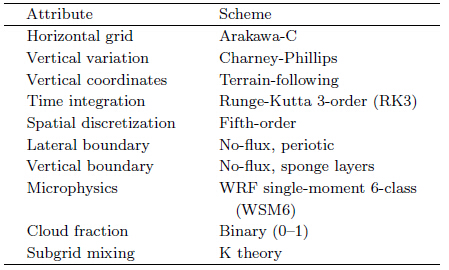
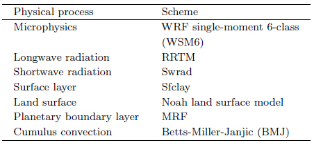
2. SP-GRAPES 2.1 The cloud resolving modelTo implement SP in GRAPES, a simplified 2DCRM is designed and developed. This is a 2Dfully compressible model with Runge-Kutta threeorder time integration scheme and a five-order spatialdiscretization scheme(RK3-5). To best fit the purpose of coupling with GRAPES, the grid configurationof the CRM is consistent with that of RK3-5, withhorizontally-staggered Arakawa-C grid and CharneyPhillips variation configuration in the terrain-followingvertical coordinates. The physical parameterizationemployed is simplistic, with only microphysics and cloud fraction under consideration. This is to facilitate the comparison of the impact of incorporatingmore or fewer model physics parameterizations.
The main characteristics of the CRM are shownin Table 1, and further details can be found in the Ap-pendix.
The performance of the CRM was evaluated byusing classical benchmark tests such as the densitycurrent, convective thermal bubble, internal gravitywaves, and idealized thunderstorm. These simulationsproved that the CRM performs well for typical atmospheric phenomenon such as convection and vortex development. The dynamic framework was thus considered robust, and qualified for high-resolution simulation. Additionally, the microphysics parameterizationwas considered adequate for cloud-scale simulation.
2.2 SP methodologyFor successfully implementing SP, harmoniouscoupling of a large-scale model and a CRM is necessary. Although the SP research was initiated since adecade ago, there has been no change in the main ideaused for coupling. As discussed in Jung and Arakawa(2005), the equations for the large-scale model in acoupled system are represented by
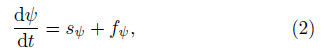
where ψ is an arbitrary prognostic variable, D=Dt =∂=∂t +U ▽, and U =(U; V;W)represents the windcomponents resolved by the large-scale model. Theterm Sψ represents the source of ψ explicitly resolvedby the large-scale model, and Fψ represents the sourceof ψ due to the processes that can only be resolved bythe CRM, i.e., the forcing term. Similarly, the CRMequation can be represented aswhere ψ is an arbitrary prognostic variable, and d=dt = ∂=∂t + u ▽, u =(u; v;w)represents thewind components resolved by the CRM. The terms sψ and fψ represent the source of ψ explicitly resolved bythe CRM, and the source of ψ due to the processes(forcing)represented by the large-scale model, respectively. The two models are coupled together primarilyby the two forcing terms Fψ and fψ.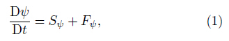
Studies following that of Jung and Arakawa(2005)focused on the configuration of the CRM withinthe grid of the large-scale model. The original methodproposed by Grabowski and Smolarkiewicz(1999) and Grabowski(2001)places a 2D CRM in an east-westor south-north direction within the large-scale grid, wherein the CRM is located only near the center ofthe grid as a sample and does not traverse the entirearea of the grid. In such a case, the lateral boundarycondition of the CRM is periodical; thus, the cloudprocesses are limited within the area of the grid, and large-scale advection primarily relies on the forcing effect provided by the large-scale model.
A later study by Arakawa(2004)proposed twodesigns. The first design was to place two 2D CRMsin both east-west and south-north directions within the grid; although the CRM in the center of the gridis pseudo 3D, it still does not traverse the entire areaof the grid. The second design was to exp and the areaof the 2D CRM to the entire grid area in the direction of east-west or south-north, and exchange datafrom adjacent CRMs through the boundary, withoutassistance from the large-scale model. The second design was then implemented in the work of Jung and Arakawa(2005) and preliminary results showed a certain improvement.
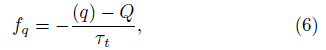
The question now is how to formulate the forcing terms Fψ and fψ. If the periodical lateral bound-ary is adopted in the CRM and no data are exchanged between the adjacent CRMs, the forcingterms of thermal-dynamic variations(potential temperature and water vapor)Q provided by the CRM tothe large-scale model can thus be represented by
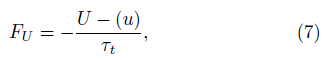
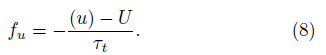
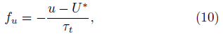
where \()" denotes the horizontal average. Additionally, according to Jung and Arakawa(2005), the counterpart forcing term of thermal-dynamic variations(potential temperature and water vapor)q providedby the large-scale model to the CRM can be repre-sented asAnother approach used is similar to the idea ofnudging, as discussed in Khairoutdinov et al.(2005), which defines and where Τt is the nudging timescale. For the zonal windcomponents U and u, one approach is then used tolink the two models, making them force each other bythe terms and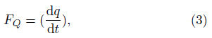


A further approach is to ignore the forcing termsof momentum because of the unrealistic representationof momentum in the 2D CRM(Khairoutdinov et al., 2005).
sHowever, if the adjacent CRMs exchange databetween each other, the forcing terms of thermaldynamic variations(potential temperature and water vapor)Q provided by the CRM to the large-scalemodel can be represented by
and the forcing term fu provided by the large-scalemodel to the CRM iswhere U* is the zonal wind component interpolatedto the grids of the CRM, and the other forcing termsremain unchanged. 2.3 Construction of SP-GRAPES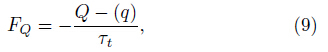
Considering that this is a preliminary study thatapplies SP to a weather model, we select a comparatively simple coupling scheme to ensure that everystep is solid. In every grid of GRAPES, a simplified2D CRM is placed in the center of the grid in theeast-west direction with a periodical lateral boundarycondition. The CRM traverses the entire area of thegrid. However, no data are exchanged between adjacent CRMs through the boundary. Because the momentum simulated by the 2D CRM is unrealistic, weignore the forcing effect of zonal wind as thus used by Khairoutdinov et al.(2005). The forcing terms under consideration are those made by thermal-dynamicvariations(potential temperature and water vapor)Q and q, which prompt the CRM and GRAPES to mutually force each other and can be represented by Eqs.(5) and (6), with a nudging timescale of 3600 s(further details pertaining to this nudging method are discussed in Khairoutdinov et al.(2005)). The forcingrelated to momentum is ignored here because of theabove-mentioned reason.
When GRAPES is initialized, the vertical pro-files of thermal-dynamic variations are entered in theCRM, and the perturbation of thermal temperature is introduced as
where R and om{0, 1} represents r and om numbersranging from 0 to 1, and △θ = 2 K, thereby forming a r and om perturbation ranging from {1 to 1 K.The forcing terms F and f are updated and work after the GRAPES time step of △t. The output of theCRM is stored after every △t to ensure the smooth operation of the CRM within the following time step ofGRAPES. Through this configuration, the CRM and GRAPES are able to mutually force each other. Ar and om perturbation will thus develop with the integration of time, and finally cloud-scale characteristicswill evolve.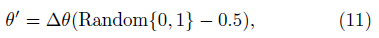
To evaluate the impact of coupling the CRM withGRAPES, we constructed SP-GRAPES in two phases.In the first phase, the SP module(the simplified 2DCRM)replaced the original microphysics and cumulusmodules in GRAPES. However, cloud fraction simulated by the CRM did not feed back to GRAPES, and instead cloud fraction used for computing the radiative heating was provided by GRAPES. This phasewas considered to be the basic phase, which considered only the microphysics processes. In the secondphase, cloud fraction module of the CRM worked as apart of the SP, implying that cloud fraction was computed by the CRM and it then fed back to GRAPES.The physics of the CRM was therefore developed to become more complete, and we considered that theCRM would deliver an optimum performance for containing a fully integrated physics package.
3. Preliminary resultsThe SP-GRAPES presented in this paper is basedon GRAPES-Meso 3.3.2.5, which is a regional weathermodel. We selected a regional model instead of aglobal model for the following reasons. First, SP canincrease the model resolution over a particular regionof interest. Traditionally, domain nesting is used toincrease model resolution in regional models, the mostfamous of which is the Weather Research and Forecasting Model(WRF). Recently, the use of varyingmesh technique has enabled realization of finest reso-lutions even in a global model such as the Model forPrediction Across Scales-Atmosphere(MPAS-A; Skamarock et al., 2012). However, both domain nesting and mesh varying have problems in selection of appropriate physical parameterizations. For example, it is hard to decide the horizontal resolutions of thenested domains for cumulus parameterization in a regional model, and with the multi-scale model MPASA, multi-scale physical parameterizations need to bedeveloped. In contrast, SP can unify the scale of themodel to the cloud scale, rendering the selection ofphysical parameterizations fixed to those on the cloudscale. Therefore, with the SP method, the resolutionof a regional model can be increased without scarifyingthe effectiveness of some model physical parameterizations. Second, SP in a regional model is practical sinceit is not foreseeable for global models' resolution to befiner than mesoscale over a certain period of time. Atpresent, results from this paper can be used as reference for studies about the use of SP in GCMs, untilglobal CRMs become more affordable.
Because SP-GRAPES runs are computationallyvery expensive, we chose only a single case(the Beijing \7.21" heavy rainfall event)to conduct a numeri-cal experiment for verifying its performance. The Beijing \7.21" heavy rainfall refers to a century precipita-tion event that happened in Beijing during 21{22 July2012. The event involved multi-scale characteristics, and the main cause of the huge amount of precipitation was the plentiful supply of water vapor. In addition, there was frequent development of mesoscaleconvective systems(MCSs), which persisted in time and space. Moreover, there was strong convergenceshear line ahead of the cold front, which enhanced theconvergence of water vapor and air mass in the lowerlayers of the MCSs and enabled the release of unstable energy(Sun et al., 2013; Ran et al., 2014). Thisprecipitation event was therefore considered a goodexample to verify the performance of a model, and asimulation of the extreme precipitation event with SPGRAPES was thus undertaken, focusing particularlyon the model's ability to simulate the triggering and the development of the MCSs.
3.1 Design of numerical experiments3.1.1 Control runA control run(CTL-run) and an SP-run required huge computational resources, and thus, thedomain of these runs was limited to a moderatesized region covering North China with its center lo-cated over Beijing. The geographic coordinates ofthe left corner(33±N, 108±E) and 100 × 100 gridpoints were used, and the resolution was 0.15±(approximately 15 km). The domain therefore was33±{ 47.85±N, 108±{122.85±E. The background datawere obtained from the NCEP Final Analysis(FNL;http://rda.ucar.edu/datasets/ds083.2/). The timestep was 90 s, the initial time was 0000 UTC 21 July2012, and the forecasting range was 24 h.
The CTL-run adopted the default settings of theGRAPES physical parameterization schemes. The microphysics scheme was WRF single-moment 6-class(WSM6) and the cumulus scheme was Betts-MillerJanjic(BMJ). A complete description of the modelphysics can be seen in Table 2.
Because the SP method has a high-computationalconsumption, we applied the SP method only inBeijing area. Based on the configuration of the CTL-run, the cumulus and microphysics schemes were thenshut down in Beijing area(39.15±{41.40±N, 115.05±{118.05 ±E). The initial time of the simulation wasagain 0000 UTC 21 July 2012 and the length of themodel run was 24 h. Because the horizontal grid interval for GRAPES was approximately 15 km and timestep was 90 s, and those for the CRM were 500 m and 0.1 s, the CRM was advanced 900 steps within one time step of GRAPES.
As previously mentioned, the SP-runs were conducted in two phases: Phase I and Phase II. Phase IIincluded feedback of cloud fraction simulated by theCRM, but Phase I did not include this information.The following subsections show verification of the precipitation forecast from both phases.
3.2 Verification of precipitation forecast3.2.1 Observational dataHourly precipitation data from \CMORPH fusionprecipitation products on a 0.1± grid(version 1.0)"provided by the Meteorological Data Research O±ce(MDRO)of the National Meteorological InformationCenter(NMIC)of China were chosen as the observational data for verifying the results of both CTL-run and SP-run. To enable a reasonable comparison withthe predicted precipitation, the observations were interpolated to the 0.15± mesh grid as that of the SPGRAPES runs.
3.2.2 Distribution of precipitation3.2.2.1 CTL-runFigure 1 shows the spatial distributions of theamount of observed and predicted 24-h cumulativeprecipitation between 0000 UTC 21 and 0000 UTC 22 July 2012. The CTL-run roughly captured the shapeof the rainb and extending from southwest to northeast, with precipitation centers mainly located overBeijing. However, the observed maximum precipitation occurred southwest of Beijing, but it was locatedsoutheast of Beijing and at the junction of Hebei and Tianjin in the CTL-run. In addition, the observedmaximum precipitation amount for Beijing(39.15±{41.40±N, 115.05±{ 118.05±E)was 358.3 mm, whileCTL-run produced a maximum precipitation amountof 238.1 mm.
 |
| Fig. 1. Distributions of the amount of(a)observational 24-h cumulative precipitation and (b)that from the CTL-run(mm day-1). The black box denotes the area of Beijing(39.15±{41.4±N, 115.05±{118.05±E). |
To investigate the reason for the differences inthese results, we split the total precipitation into twoparts: grid-scale(non-convective)precipitation and subgrid-scale(convective)precipitation, as shown inFig. 2. The figure reveals that in the Beijing region, the BMJ cumulus scheme did not produce much precipitation. This is significantly different from the observation since convective precipitation is an impor-tant component of total precipitation in Beijing, assuggested by previous studies(Sun et al., 2013; Ran et al., 2014). As there was not much convective precipitation from the BMJ scheme in the CTL-run in theregion of Beijing, it is likely that the water vapor wasadequately consumed within the process of advection from west to east. This could be the reason for thelocation of the maximum precipitation east of the observation and for the precipitation to be less than thatof the real data. If the model could capture the cumulus convective processes near Beijing, convective precipitation would therefore increase and ultimately thetotal precipitation would also increase.
 |
| Fig. 2. Grid-scale(non-convective)precipitation(a) and subgrid-scale(convective)precipitation(b)from the CTL-run(mm day-1). The Black box represents the area of Beijing. |
Replacing the original cumulus scheme and microphysics scheme with an SP scheme in the Beijingregion during the SP-run, the model was initiated at0000 UTC 21 July 2012 and was integrated for 24 h.The result delivered both positive and negative effects.
Figure 3 compares distributions of hourly precipitation from the observation, CTL-run, and SP-runbetween the 11th and 14th hours, which is approximately the time period when the Beijing \7.21" heavyrainfall was generated, developed, and matured. InFig. 3, the generation time and the development extent of the heavy rain in the SP-run are much closerto the observation than those in the CTL-run. However, the locations of heavy rain do not exactly matchbetween observation and simulation.
 |
| Fig. 3. Distributions of hourly precipitation(mm h-1)from the(a1{a4)observation, (b1{b4)CTL-run, and (c1{c4)SP-run, from the 11th to 14th hours. |
Figure 4 shows the 850-hPa water vapor transportdifferences at the 12th hour between the NCEP FNLdata and the CTL-run(CTL{FNL) and between FNL data and the SP-run(SP{FNL). Positive values indicate larger water vapor transport in the simulations(CTL-run and SP-run)than in the FNL data, while anegative value implies the opposite.
 |
| Fig. 4. Differences in 850-hPa water vapor transport at the 12th hour between(a)NCEP FNL data and CTL-run(CTL{FNL), and (b)FNL data and SP-run(SP{FNL). Vectors represent the differences in 850-hPa wind ¯eld(m s-1);shadings represent the differences in 850-hPa water vapor flux(g cm-1 hPa-1 s-1). |
From Fig. 4, it is seen that the simulation of water vapor transport has deviated from the FNL datato a certain extent at the 12th hour in both CTL-run and SP-run, but in some local areas(south rim of Beijing at the left-bottom corner in the black box), thesimulation of SP-run is superior to that of CTL-run.Notably, in the upper-right corner of the domain, thebias of SP-run is larger because the coupling schemeof the SP ignores the feedback of the wind field. Inother regions, simulation of the wind components inSP-run is similar to that in CTL-run.
The average vertical profiles of potential temperature, water vapor mixing ratio, and vertical velocityin the area within 50 km around(40±N, 116±E)atthe 12th hour are shown in Fig. 5. With referenceto the 12th hour precipitation in Fig. 3, it can beinferred that only a small amount of precipitation isobserved in this area, and both SP-run and CTL-runproduced too much precipitation. Figure 5 also revealsa problem with the model simulation compared withthe FNL data in terms of the thermodynamic fields:damper and warmer in the lower layers and colder in the upper layers.
 |
| Fig. 5. Differences in(a)potential temperature(K), (b)water vapor mixing ratio(g kg-1), and (c)vertical velocity(ms-1)between the averaged results of CTL-run and SP-run with the FNL data in an area within 50 km around(40±N, 116±E)at the 12th hour. |
Figure 5 also shows that SP-run seems slightlysuperior to CTL-run in the simulation of average potential temperature, water vapor mixing ratio, and vertical velocity, compared to the FNL data(obser-vation). The reduction in the potential temperaturebias is more obvious than in the water vapor mixingratio bias, and in particular, in the layer between 5 and 13-km altitudes, the bias is reduced by up to 0.5.For the water vapor mixing ratio, the bias is mostly reduced by approximately 0.3 g kg-1. In the profile ofvertical velocity below 10 km, SP-run also has a distinct positive effect compared with CTL-run, yet theimpact of SP-run becomes negative from 10 to 17 km.Overall, the bias between SP-run and observation islargely reduced when compared with CTL-run for allverified data, except for wind speed above 10 km. Thisresult implies a positive impact on model simulationsby the SP method.
In summary, the simulation of water vapor trans-port in SP-run is superior to that of CTL-run in thelower layers, and the bias of thermodynamic profiles issmaller in certain local areas. This probably explainswhy the simulation of hourly precipitation in the SP-run is better than that in the CTL-run(Fig. 3).
The SP method produces a heavy rainfall belt inthe south rim of Beijing which is similar to that ofthe observation, and the maximum value is 405.7 mm, much closer to the observation than that of CTL-run(Fig. 6). However, the precipitation is centered in Bei-jing as a whole. Because the SP method was applied ina quite limited area, the slightly improved simulationof the precipitation location and amount near Beijingleads to a larger bias in the upper-right corner in Fig. 6.
 |
| Fig. 6. As in Fig. 1, but for a comparison between(a)the observation and (b)the result of the SP-run. |
To complement the information presented above, a statistical verification of the amount of 24-h cumulative precipitation is presented below.
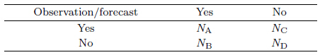
3.2.3 Statistical verification 3.2.3.1 MethodologyIn this section, the 24-h cumulative precipitation(R)is classified into five categories: slight rain(R >0.1 mm), moderate rain(0.1 > R > 10.0 mm), heavyrain(10.0 > R > 25.0 mm), rainstorm(25.0 > R >50.0 mm), and heavy rainstorm(50.0 > R > 100.0mm). The precipitation forecast is verified with abinary classification test(Table 3), where NA repre-sents the number of stations in which both the forecast and observation show precipitation, NB represents thenumber of stations in which forecast shows precipita-tion but the observation does not, NC represents thenumber of stations in which the forecast shows no pre-cipitation but the observation does, and ND representsthe number of stations in which both forecast and ob-servation show no precipitation. The descriptions ofthe statistics variable TS, PO, NH, Bias, EH, and ETSare given in Table 4.

For a forecast result of precipitation being greaterthan 0.1 mm(GT 0.1 mm hereafter), Fig. 7 shows that the CTL-run has a high TS score. The PO, NH, and Bias scores are low(below 0.2, 0.1, and 0.2, respectively), and the EH and ETS are also acceptable(above 0.8 and 0.5, respectively). However, for forecast levels of GT 10.0, GT 25.0, GT 50.0, and GT100.0 mm, the scores decrease as a whole, except forthe EH score. Interestingly, the forecast of GT 100.0mm level is overall better than that of GT 50.0 mmlevel, and the EH tends to improve when the level ofprecipitation rises.
 |
| Fig. 7. Statistical verifcation of 24-h cumulus precipitation forecast for the CTL-run(CTL)(solid line) and the SP-run(SP)(dotted line).(a)TS, (b)PO, (c)NH, (d)Bias, (e)EH, and (f)ETS. |
Comparison of the result of the SP-run and CTL-run shows that the TS and ETS scores of the SP-runrise by 0.01 to 0.02 at a precipitation level of GT 50.0mm and maintain this level at GT 100.0 mm, whereasthat for the CTL-run does not. An explanation forthis can be found in the scores of PO, NH, and Bias.The PO of the SP-run at levels of GT 50.0 mm and GT 100.0 mm are lower than those of CTL-run. Inaddition, the PO and Bias at a level of GT 50.0 mm are also slightly lower whereas the NH and Bias scoresrise for GT 100.0 mm level. However, because the areawhere the SP method is applied is quite limited, thereis no obvious impact on other levels in this experiment.
3.3 Verification of cloud fraction3.3.1 The need for verification of cloud fractioBefore we verify the simulation of cloud fractionin SP-run, determining the extent of GRAPES sensitivity to cloud fraction is necessary, and to achievethis, a simple sensitivity test is conducted. The modelphysics setting is the same as that used in the \7.21"heavy rain experiment mentioned above in Table 2, and the resolution of the model is also 0.15°× 0.15°with grid numbers of 481 × 341. The domain coversthe entire East Asia(4°-55°N, 73°-145°E).
The sensitivity test is conducted by comparingthe CTL-run with a run where the cloud is removedat every step(NoCloud-run). The original cloud fraction scheme is selected in the CTL-run; the model isinitiated at 0000 UTC 20 July 2012 and is run for72 h. In the NoCloud-run, cloud fraction is set tozero at every step throughout the domain. No otherconfigurations are changed in the NoCloud-run. Notably, cloud fraction in GRAPES is a variable thatcan only be employed by the radiation scheme; thus, the effect of deleting cloud fraction has the effect ofmaking clouds \transparent" to radiation. Therefore, this deletion only directly infuences the calculation ofradiation and any infuences on other variables are indirect and occur in the process of time integration.
Figure 8 shows the differences in surface netshortwave radiation, surface temperature, surface heatflux, and the 10-m wind field between CTL-run and NoCloud-run at the 54th hour. It shows that cloudfraction has a direct impact on the surface net shortwave radiation, and that the instantaneous differencebetween the clear area and the cloudy area is above 200 W m-2. Because of the indirect impact of cloud frac-tion, the surface temperature and heat flux also changeby more than 4℃ and 50 W m-2, respectively. Additionally, the 10-m wind field is also affected becauseof changes in the thermodynamic condition of the underlying surface. The sensitivity experiment with and without cloud reveals that the difference in 10-m windspeed reaches 1 m s-1 in the cloudy area, which issignificantly large, considering that the 10-m wind velocity is normally of the magnitude of 5 m s-1. Thisresult suggests that the 10-m wind field is sensitive tocloud cover.
 |
| Fig. 8. Diferences in(a)surface net short wave radiation(W m-2), (b)surface temperature(K), (c)surface heat flux(W m-1), and (d)10-m wind feld(m s-1)between the CTL-run and the NoCloud-run at the 54th hour. |
In summary, GRAPES shows su±cient sensitivityto cloud fraction. The variation in cloud fraction directly infuences surface radiation and indirectly infuences the thermodynamic fields(such as surface temperature and surface heat flux)in lower layers, and istherefore also able to infuence the circulation in thelower layers. Despite the fact that cloud fraction is not a forecast variable in GRAPES, it is able to indirectly affect other variables. Thus, considering the accuracy of cloud fraction simulation is necessary(Zheng et al., 2013). In light of this, the SP-run-II was conducted for the following reasons: to feed back cloudfraction simulated by the CRM to GRAPES; to verifythe simulation of cloud fraction distribution, and recheck the result of precipitation forecast. Performingthis would move us closer to achieving our target ofobtaining a physics coupler, as mentioned in Section1.
3.3.2 Distribution of total cloud fractionFigure 9 shows the FY2 satellite cloud image at0000 UTC 22 July 2012. A cloud belt was distributedfrom southwest to northeast of the domain, and wasthe thickest in Sh and ong. The southeastern part ofBeijing was also under cloud cover.
 |
| Fig. 9. FY2 satellite cloud image at 0000 UTC 22 July2012. The domain and the black box are the same as thosein Fig. 1. |
Figure 10 shows distributions of the total cloudfraction simulated in CTL-run and SP-run. The total cloud fraction is calculated as the vertical maxi-mum of cloud fraction in the grid column. The reason for choosing the maximum method for calculatingtotal cloud fraction is that the simulation was onlycompared with the FY2 satellite cloud image. Thisimage was recorded by the satellite(observing fromspace), and was calculated on the basis of the maximum method, because once there is a high value of cloud fraction over some area, the observed result doesnot differ greatly whether cloud cover is present or not.
 |
| Fig. 10. Distributions of total cloud fraction simulated in the(a)CTL-run and (b)SP-run. The total cloud fraction iscalculated as the vertical maximum of cloud fraction in the grid column. The domain and the black box are the same asthose in Fig. 1. |
From Fig. 10, we can see that the CTL-run failsto simulate the thick cumulus to the southeast of theBeijing area. The model result shows that the region isbasically clear with some cumulus in the northeasterncorner of the domain. In contrast, the SP-run showsthick cumulus in most of the Beijing area. When compared with the FY2 cloud image, the result of SP-runis seen to be in agreement with that of the observa-tion, although there is too much cloud fraction in thenorthwestern corner of the domain. Therefore, theapplication of the SP method is able to improve thesimulation of cloud fraction.
3.4 Precipitation forecast SP-run-IITo determine whether the feedback of cloud fraction could have a positive impact on the precipitationforecast, the precipitation forecast results from SP-run-II were verified.
Figure 11 shows the difference in 24-h cumulativeprecipitation between SP-run-I/SP-run-II and the observation. The results show that the excessive precipitation in SP-run-I is slightly reduced in SP-run-II, and that the maximum 24-h cumulative precipitationin SP-run-II is 386.0 mm, which is much closer to theobservation(358.3 mm)than that of SP-run-I(405.7mm). Additionally, the forecast error is reduced in theupper-right corner of the domain.
 |
| Fig. 11. Diferences in 24-h cumulative precipitation(mm day-1)between(a)result of SP-run-I and the observation, and (b)result of SP-run-II and the observation. |
The improvement is quite obvious in the results ofthe statistical verification. Figure 12 shows the resultsof a statistical verification of SP-run-II, and indicatesthat the forecast of 24-h cumulative precipitation isobviously improved in SP-run-II. For GT 25-mm, GT50-mm, and GT 100-mm levels, the TS and ETS scoresof SP-run-II are improved by 0.02{0.03, which is muchbetter than those of SP-run-I. The improvement of the EH score is also visible, although the improvement inPO, NH, and Bias is not so obvious.
 |
| Fig. 12. As in Fig. 7, but for the SP-run-II. |
In conclusion, the SP-run-II simulation is overall better than SP-run-I because of the use of cloudfraction feedback. In addition, the use of improvedintegrated physics in the CRM is expected to showfurther improvements to the simulation.
4. SummaryIn this paper, SP-GRAPES was constructed and preliminary results were reported. This was the firstattempt to apply the SP method to a numericalweather model in China; therefore, the simple uniform coupling approach discussed in Khairoutdinov etal.(2005)was employed. The forcing terms couplingthe CRM to GRAPES are known as nudging terms.Because of the limitation of computation resources, only a single case experiment was conducted in thisstudy to verify the performance of SP-GRAPES.
The area to which the SP method was appliedwas limited to a small region near Beijing. The heavyrainfall event occurring on 21 July 2012 was used as abenchmark case to verify the performance of the CTL-run, SP-run-I, and SP-run-II. The SP-runs were conducted in two phases: phase one(SP-run-I)was conducted without the feedback of cloud fraction sim-ulated by the CRM, while phase two(SP-run-II)usedthe feedback of cloud fraction. Some of the conclusions obtained from these numerical experiments areas follows.
The result of the SP-run-I shows that the SPmethod introduces a slight improvement to the precipitation forecast in the region of Beijing. Specifically, the time when the rain density was largest was captured more precisely, and the maximum precipitationwas closer to that of the observation. The TS scorefor a level of GT 50 mm was improved by 0.01 to 0.02.However, the location of the main precipitation beltstill deviated to the east, and the false alarm rate forGT 100-mm level was higher.
The result of the SP-run-II indicates that usingthe feedback of cloud fraction led to an evident overall improvement. The simulation for the distributionof total cloud fraction was distinctly improved and was closer to that of the FY2 satellite cloud image.This better-simulated cloud fraction had a positiveimpact on the precipitation forecast, which led to themaximum precipitation amount from SP-run-II beingcloser to the observation, and the superfuous precipitation amount found in SP-run-I was reduced to acertain degree.
A comparison of the SP-run-I and SP-run-IIshows the positive impact of unifying the modelphysics to cloud scale. A preliminary framework forSP-GRAPES was constructed. Although the perfor-mance of SP-GRAPES was found to be limited, thiswork is the first of this kind in China. SP is the firststep to realize the goal of unified model physics. Thispaper is a preliminary trial for applying the methodto a weather model. The study aims to provide areference for follow-up studies on SP in China. It isconsidered that further studies using the frameworkof SP-GRAPES are needed, and such studies shouldinclude enrichment for the model physics of the CRM, a methodology for feeding back to the dynamic vari-ables, and an algorithm to achieve a superior parallelcalculation for the SP-GRAPES.
Acknowledgments: The authors would liketo express their gratitude to Dr. Louis Wicker, Dr.Xingliang Li, Dr. Xindong Peng, Dr. HongliangZhang, and Miss Xiaohan Li for helpful discussionsrelated to the numerical techniques used in this study.We are also grateful to Dr. Dehui Chen, Dr. XueshunShen, Prof. Bin Zhu, and Dr. Qijun Liu for theircomments and suggestions.
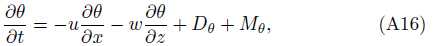
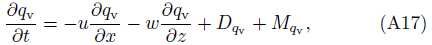
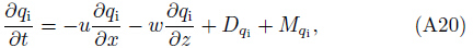
APPENDIXConstructing a Two-Dimensional Simplified Cloud Resolving Model 1. Governing equations
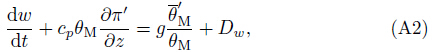
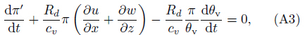
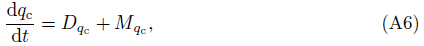
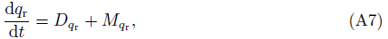
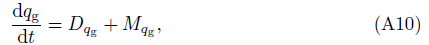
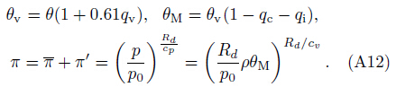
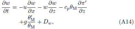
Following Durran and Klemp(1983), the govern-ing equations of the CRM are modified as below:
where and This is a two-dimensional fully compressible modelwithout the Coriolis force, and it includes momentum, pressure, thermodynamic, and moisture equations. Inthe equations, u and w are the horizontal and verticalwind component, respectively, π the Exner function, θ the potential temperature, θv the virtual potentialtemperature, θM the moist potential temperature, pthe pressure, p0=1000 hPa, and ρ the total density.The mixing ratios of water vapor, cloud water, cloudice, rain, snow, and graupel are qv; qc; qi; qr; qs; and qg, respectively. The terms D and M are contributionsfrom subgrid scale mixing and cloud microphysics, respectively. Overbar denotes the reference state of variables, while apostrophes denote the perturbation.2. Model discretization 2.1 Grid setting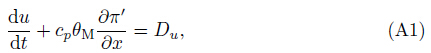


The use of SP requires that the vertical grid ofthe CRM is consistent with that of GRAPES, and ahigh resolution is always needed in a CRM; therefore, the Arakawa-C staggered grid(Arakawa and Lamb, 1981) and the Charney-Phillips vertical variable setting(Charney and Phillips, 1953)are employed tomake the model suitable for simulation of a strongvortex and mesoscale or cloud-scale circulations.
Four types of grid(u-grid, v-grid, π-grid, and w-grid)are defined as in Fig. A1, and all variables arestored on different types of grids as below.
 |
| Fig. A1. Grid setting of the CRM. The thick line outlinesthe boundary of the domain. The indexes(such as its, ite, kts, and kte)indicate the positions of the grids. |
Horizontal wind component is stored on the u-grid; vertical wind component w, potential tempera-ture θ, and water substances q are stored on the w-grid; Exner function π is stored on the π-grid; v-gridis a virtual grid type with no variables stored thereon.It is used only when interpolation is needed.
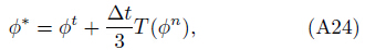
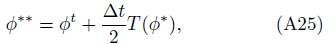
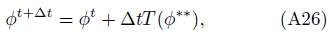
2.2 Time integration schemeThe governing equations may be written in trans formed forms as


To pursue a high performance of time integra-tion, the sophisticated Runge-Kutta 3(RK3)(Wicker and Skamarock, 2002)is adopted. For all the prog-nostic variables of the CRM, Φ =(u;w; π′; θ; qv; qc;qr; qi; qs; qg), the tendency terms can be written as
and the solution Φ(t)is advanced to Φ(t+∂t)in threesteps:where △t is the time step of the CRM.2.3 Advection scheme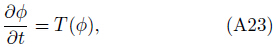
To conserve mass and momentum, the advectionterms of the governing equations are configured in fluxform as below(taking x-direction as example):
The fluxes can be spatially discretized in the 2nd-, 3rd-, 4th-, 5th-, and 6th orders as listed below,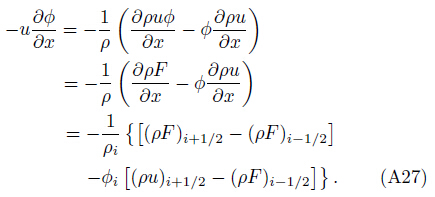
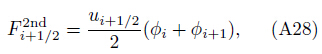
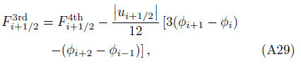
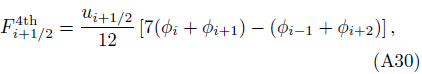
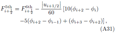

According to Wicker and Skamarock(2002), oddordered schemes perform better(in terms of stability)than even-ordered schemes. Thus, in practice, the CRM takes the RK3-5(RK3 time scheme with 5-orderspatial scheme)spatiotemporal discretization schemeas its default setting. Additionally, a reducing approximation alternative of the RK3-2 scheme is also appliednear the boundaries of the domain when required.
2.4 Boundary conditionsSome of the regular boundary conditions availablein the CRM are presented below.
No-flux: The no-flux boundary condition is alsocalled the \symmetric boundary condition." Variablesin the ghost zone take values assuming they are in amirror:
where xb is the position of the boundary, u is the hor-izontal wind component, and Φ represents all othervariables.

Periodic: The periodic boundary condition is of-ten used in the lateral direction. It makes the domaincyclic to avoid a complex treatment of the boundary.It may be configured aswhere Lx is the length of periodic boundary, and Φrepresents all other variables.Sponge layers: To absorb vertically propagatedgravity waves, when Φ =(u;w; θ; qv; qc;qr; qi; qs; qg)iscalculated, sponge layers are imposed as Rayleigh layers:
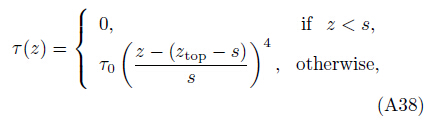
where Φ is the reference state of the variables, and Τ(z)changes with the position, which is defined aswhere z is the height, ztop the top height of the model, s the thickness of Rayleigh layers, and Τ0 the inverseof the timescale(constant). 3. Model physics3.1 Microphysics scheme
For a moist atmospheric model, parameterizing the microphysics processes is always considerednecessary because they are always on subgrid scale.The WRF single-moment 6-class microphysics scheme(WSM6) (Hong and Lim, 2006) is adopted in theCRM.
WSM6 is one of the essential microphysicsschemes in the current versions of the Weather Re-search and Forecasting Model(WRF). It was devel-oped and evolved from the WSM3(Hong et al., 2004) and WSM5( Lim and Hong, 2005). It contains mi-crophysics processes between water vapor(qv), cloudwater(qc), cloud ice(qi), rain(qr), snow(qs), and graupel(qg). We believe that WSM6 is su±ciently so-phisticated to represent microphysics on a cloud scale.
3.2 Cloud fraction schemeThe binary cloud fraction scheme is used to represent the grid cloud fraction of the model, and can bepresented as follows:
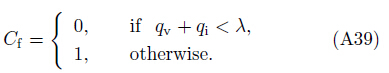
In this scheme, the cloud fraction(Cf)of eachgrid is either 0 or 1. If the sum of the mixing ratioof cloud water(qv) and the mixing ratio of cloud ice(qi)is over a threshold λ(e.g., λ = 1:0 × 10-6), thenthe cloud fraction is 1, otherwise it is 0. This simplescheme is appropriate here because the resolution ofthe cloud model is su±ciently fine.
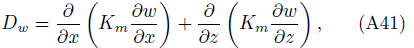
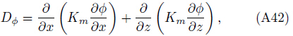
3.3 Subgrid mixing schemeThe subgrid mixing process(or turbulence)is simply parameterized using K theory:
where Φ =(θ; qv; qc;qr; qi; qs; qg).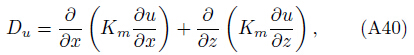
| Arakawa, A., 2004: The cumulus parameterization prob-lem: Past, present, and future. J. Climate, 17, 2493-2525. |
| Arakawa, A., and V. R. Lamb, 1981: A potential enstro-phy and energy conserving scheme for the shallow water equations. Mon. Wea. Rev., 109, 18-36. |
| Charney, J. G., and N. A. Phillips, 1953: Numerical integration of the quasi-geostrophic equations for barotropic and simple baroclinic flows. J. Meteor., 10, 71-99. |
| Chen Dehui, Xue Jishan, Yang Xuesheng, et al., 2008: The overall design of the new genera-tion global/regional multi-scale unified numerical weather prediction system GRAPES. Chin. Sci. Bull., 53, 2396-2407. |
| Durran, D. R., and J. B. Klemp, 1983: A compressible model for the simulation of moist mountain waves. Mon. Wea. Rev., 111, 2341-2361. |
| Grabowski, W. W., 2001: Coupling cloud processes with the large-scale dynamics using the cloud-resolving convection parameterization (CRCP). J. Atmos. Sci., 58, 978-997. |
| Grabowski, W. W., 2003: Impact of cloud microphysics on convective-radiative quasi equilibrium revealed by cloud-resolving convection parameterization. J. Climate, 16, 3463-3475. |
| Grabowski, W. W., 2006: Impact of explicit atmosphere-ocean coupling on MJO-like coherent structures in idealized Aqua Planet simulations. J. Atmos. Sci., 63, 2289-2306. |
| Grabowski, W. W., and P. K. Smolarkiewicz, 1999: CRCP: A cloud resolving convection parameteri-zation for modeling the tropical convecting atmo-sphere. Physica D: Nonlinear Phenomena, 133, 171-178. |
| Hong, S.-Y., J. Dudhia, and S.-H. Chen, 2004: A revised approach to ice microphysical processes for the bulk parameterization of clouds and precipitation. Mon. Wea. Rev., 132, 103-120. |
| Hong, S.-Y., and J.-O. J. Lim, 2006: The WRF single-moment 6-class microphysics scheme (WSM6). J. Korean Meteo., 42, 129-151. |
| Jung, J.-H., and A. Arakawa, 2005: Preliminary tests of multiscale modeling with a two-dimensional frame-work: Sensitivity to coupling methods. Mon. Wea. Rev., 133, 649-662. |
| Khairoutdinov, M., D. Randall, and C. DeMott, 2005: Simulations of the atmospheric general circulation using a cloud-resolving model as a super parameter-ization of physical processes. J. Atmos. Sci., 62, 2136-2154. |
| Khairoutdinov, M. F., and D. A. Randall, 2001: A cloud resolving model as a cloud parameterization in the NCAR community climate system model: Prelimi-nary results. Geophys. Res. Lett., 28, 3617-3620. |
| Lim, J.-O.J., and S.-Y. Hong, 2005: Effects of bulk ice microphysics on the simulated monsoonal precipi-tation over East Asia. J. Geophys. Res., 110, doi: 10.1029/2005JD006166. |
| Moncrieff, M. W., 2004: Analytic representation of the large-scale organization of tropical convection. J. Atmos. Sci., 61, 1521-1538. |
| Ran Lingkun, Qi Yanbin, and Hao Shouchang, 2014: Analysis and forecasting of heavy rainfall case on 21 July 2012 with dynamical parameters. Chinese J. Atmos. Sci., 38, 83-100. (in Chinese) |
| Randall, D., M. Khairoutdinov, A. Arakawa, et al., 2003: Breaking the cloud parameterization deadlock. Bull. Amer. Meteor. Soc., 84, 1547-1564. |
| Shen Tongli, Tian Yongxiang, Ge Xiaozhen, et al., 2006: Numerical Weather Prediction. 2nd ed., China Me-teorological Press, 431-432. |
| Skamarock, W. C., J. B. Klemp, M. G. Duda, et al., 2012: A multiscale nonhydrostatic atmospheric model us-ing centroidal voronoi tesselations and C-grid stag-gering. Mon. Wea. Rev., 140, 3090-3105. |
| Sun Jianhua, Zhao Sixiong, Fu Shenming, et al., 2013: Multi-scale characteristics of record heavy rainfall over Beijing area on July 21, 2012. Chinese J. At-mos. Sci., 37, 705-718. (in Chinese) |
| Wang Bizheng, Liu Min, and Zeng Qingcun, 2005: Study on cloud system superparameterization and the method of characteristic lines in the atmospheric general circulation model. Climatic Environ. Res., 10, 638-648. (in Chinese) |
| Wicker, L. J., and W. C. Skamarock, 2002: Time-spliting methods for elastic models using forward time schemes. Mon. Wea. Rev., 130, 2088-2097. |
| Xu Guoqiang, Chen Dehui, Zhang Hongliang, et al., 2010: The impacts of time-level computation precision of physics in the GRAPES model on precipitation pre-diction. Chinese J. Atmos. Sci., 34, 875-881. (in Chinese) |
| Xu Guoqiang, Chen Dehui, Xue Jishan, et al., 2008: The optimization experiment and program design of GRAPES physical processes. Chin. Sci. Bull., 53, 2328-2434. (in Chinese) |
| Xue Jishan and Chen Dehui, 2008: The Scientific Design and Application of Numerical Weather Prediction System GRAPES. Science Press, 137. (in Chinese) Zheng Xiaohui, Xu Guoqing, and Wei Rongqing, 2013: Introducing and influence testing of the new cloud fraction scheme in the GRAPES. Chinese J. Me-teor., 39, 57-66. (in Chinese) |
| Zhu, H., H. Hendon, and C. Jakob, 2009: Convection in a parameterized and superparameterized model and its role in the representation of the MJO. J. Atmos. Sci., 66, 2796-2811. |