 2015, Vol. 28
The Chinese Meteorological Society
Article Information
- HU Zhiqun, LIU Liping, WU Linlin, WEI Qing. 2015.
- A Comparison of De-noising Methods for Differential Phase Shift and Associated Rainfall Estimation
- J. Meteor. Res., 28(2): 315-327
- http://dx.doi.org/10.1007/s13351-015-4062-6
Article History
- Received June 25, 2014;
- in final form October 8, 2014


2 Nanjing Meteorological Radar Open Laboratory, Jiangsu Institute of Meteorological Sciences, Nanjing 210008;
3 Anhui Weather Modification Office, Hefei 230031
Quantitative precipitation estimation(QPE)isone of the most important applications for weatherradar. A comprehensive review of the reliability ofweather radar QPE products was conducted by Wilson andBrandes(1979), and it discussed in detailthe sources of uncertainty associated with radar-basedrainfall estimates. These include calibration, attenuation, anomalous propagation, bright b and , beamblockage, ground clutter, spurious returns, and r and omerrors. Moreover, the variability in the relationshipbetween reflectivity(Z) and rainfall rate(R)(Z–R relations)was also discussed. Since that time, therehas been great progress in radar hardware and QPEalgorithms. Polarimetric radar can measure multiplepolarization parameters, including differential reflectivityZDR, specific differential phase KDR, and cross-correlation coefficient ρHV between two orthogonalradar returns. ZDR reflects the median drop diameter.KDR is immune to radar miscalibration, attenuationin precipitation, and beam blockage, while ρDRcan significantly improve the radar data quality, distinguishingrain echoes from the radar signals causedby other scatters such as snow, ground clutter, insects, birds, chaff, etc.(Zrnic and Ryzhkov, 1996; Krajewski et al., 2010). In recent years, radar meteorologistshave paid more attention to the polarimetric radar and its QPE products.
By combining a variety of polarization observationalparameters, several QPE algorithms such asR(ZH), R(ZH, ZDR), R(ZH, ZDR, KDP), and R(KDP)have been investigated in the past decades(Bringi and Chandrasekar, 2001; Liu et al., 2002; Brandes et al., 2003; Ryzhkov et al., 2005; Hu et al., 2010). However, since polarimetric variables are the difference betweenhorizontal and vertical polarization, their values areone order of magnitude smaller than those measuredfrom only a single polarization direction. Moreover, polarimetric variables are easily influenced by noise, which needs to be removed before generating the polarimetricradar-derived rainfall estimation. For example, Jameson(1991) and Ryzhkov and Zrnić(1995)investigated the relationship between rainfall and polarimetricparameters. Their results indicated thatR(KDP, ZDR)was better relative to R(ZH), R(ZH, ZDR), and R(KDP)for moderate to heavy rain rates, however, KDP and ZDR needed to be smoothed forgreater accuracy of R(KDP, ZDR)relative to R(KDP).Carey et al.(2000)developed a propagation correctionalgorithm utilizing the differential propagation phase(ΦDP) and tested this algorithm using experimentaldata from the C-b and polarimetric radar. Their resultshowed that the algorithm greatly reduced theerror of R(KDP, ZDR). Cifelli et al.(2011)presentedan optimization algorithm to estimate rainfall on thebasis of ZH, ZDR, and KDP, which performed betterin both tropical and extratropical regions. Moreover, the US National Severe Storms Laboratory(NSSL)conducted an operational demonstration for the polarimetricradar KOUN, and tested the reliability ofKOUN radar QPE for different seasons and rain typesusing a large dataset. The hourly rain estimate errorsusing polarimetric QPE were shown to decreasesignificantly compared to the conventional nonpolarimetricQPE(Ryzhkov et al., 2005). The US NationalWeather Service(NWS)upgraded the WeatherSurveillance Radar-1988 Doppler(WSR-88D)networkwith polarimetric capability in 2013.
The polarimetric parameter ZDR is easily influencedby radar hardware such as the difference betweenthe two orthogonal polarization directions ofantenna gains, rotary joints, waveguides, and receivers(Melnikov et al., 2003). Thus, correction for ZDR systembias is extremely complicated and a small errorof ZDR can possibly cause a large bias of ZDR-basedQPE. In addition, the reliability of ZDR-based QPEis greatly affected by attenuation, especially for heavyrainfall. KDP, which has been used more widely for polarimetricradar-derived QPE, is the slope of the ΦDPprofile and is noisy and unstable in measurement, especiallyfor light rain. Thus, pretreatment of ΦDP iscrucial for KDP estimate quality(Liu et al., 2013).
In recent decades, many ΦDP de-noising methodshave been developed for increasing the accuracyof R(KDP). Sachidan and a and Zrnić(1987)presentedan analysis of the accuracy of QPE from observed data and a simulation procedure, which indicated that errorscaused by sidelobe contamination significantly affectΦDP data. As such, large scale averaging is requiredto obtain reasonably accurate rain rate estimates.Chandrasekar et al.(1990)focused on theerror structure of KDP, and simulated r and om errorsin ZH, ZDR, and KDP, which suggested that R(KDP)is stable and insensitive to system calibration.As KDP is crucial in polarimetric radar-derivedrain estimates, radar meteorologists have for manyyears investigated how to obtain accurate KDP datafrom ΦDP. An iterative filtering technique has beendeveloped to estimate KDP, which can separate bothΦDP and the differential backscatter phase shift δ fromcomplicated echoes(Hubbert et al., 1993; Hubbert and Bringi, 1995). Ryzhkov and Zrnic(1996)presented analgorithm that uses KDP exclusively, and suggestedthat R(KDP)can be successfully applied to low rainrates, however, the ΦDP fitting interval needs to beadjusted. May et al.(1999)described a KDP estimationalgorithm, for which R(KDP)produces higherquality data than R(ZH)for moderate to high rainrates. Gorgucci et al.(1999, 2000)similarly describedan algorithm to correct bias in the estimation of KDPin nonuniform rainfall paths and evaluated KDP-basedrainfall algorithms for different pathlengths. With thedevelopment of polarization radar, and the recent applicationof a new mathematical method, ΦDP and KDP process methods are constantly developed. Wang and Chandrasekar(2009)presented a robust algorithmto process ΦDP, which is able to remain in sync withthe spatial gradients of rainfall and produce a highresolutionKDP.Recently, an extended Kalman filter frameworkwas proposed, which determines rain-rate via a relationshipbetween R, KDP, and ZDR(Schneebeli and Berne, 2012; Grazioli et al., 2014). Vulpiani et al.(2012)demonstrated that R(KDP)has a more seasonalrelationship than R(ZH), except for the analyzed winterstorm. To estimate high-resolution KDP, Hu et al.(2012)developed an algorithm that can smoothen ΦDPas well as a synthetic ZH/KDP-based rainfall estimationmethod. They showed that the accuracy of R(ZH, KDP)is higher than the traditional R(ZH)methodwhen the rain rate is larger than 5 mm h−1. Giangr and eet al.(2013)presented an application of linearprogramming for physical retrievals, in order toprocess measured ΦDP by developing realistic physicalconstraints for the monotonicity and polarimetricradar self-consistency. Hu and Liu(2014)introducedwavelet analysis into the ΦDP de-noising process and further addressed a ΦDP penalty threshold strategybased on the attribution of weather echoes.
A variety of ΦDP de-noising methods are usedextensively, yet there remains a lack of comprehensivecomparative analysis of these de-noising methods and their influences on KDP-based QPE. In thepresent study, several new ΦDP de-noising methodsare introduced in Section 2. In Section 3, a simulatednoisy ΦDP profile is constructed and filtered with these and other traditional methods. The bias is comparedwhere KDP is calculated from the simulated ΦDP withvarious de-noising methods. In Section 4, an observedΦDP radial profile is selected as an example to determinethe differences between raw and de-noised data.In Section 5, KDP-based rainfall estimates are verifiedagainst rain gauge measurements to evaluate theability of the ΦDP de-noising methods. Finally, theconclusions and discussion are given in Section 6.2. Description of de-noising methods
With exception of the traditional running average and median filter methods, a host of new algorithmshave also been applied into the ΦDP de-noising process.The following three methods, finite-impulse responsefilter(FIR), Kalman filter, and wavelet analysis, havebeen proved effective in removing ΦDP noise.2.1 Finite-impulse response filter
An FIR filter system function H(z)may be givenas follows,
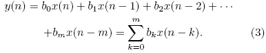
where coefficients b0, b1, · · ·, bm−1 represent the systemunit impulse response h(0), h(1), · · ·, h(m−1); nis the time or the coordinates in space or distance, and indicates the ordinal number of gates in a radar radial;m is the filter window width, and here also refers tothe smoothing gate number in a radar radial. After asignal x(n)is processed with FIR, the output y(n)isshown aswhere “*” denotes the convolution. The FIR systemcan be calculated from the following difference equation,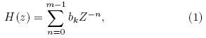

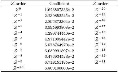
Proakis and Manolakis(1988)used symmetric20th-order associated coefficients in the complex variableZ(Table 1). This method was used to smooththe ΦDP radial profile for both the German AerospaceResearch Institute’s C-b and radar and the NCAR CP-2 radar(Hubbert et al., 1993; Hubbert and Bringi, 1995). In this study, the same coefficients in Table 1were substituted into bk in Eq.(3)to smooth the ΦDPradial profile.
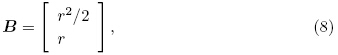
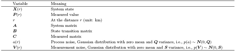
For the Kalman filter, the observational data areregarded as an output from a state equation and theleast mean square error is used as an optimal estimationcriterion to estimate the state vector of the origi nal system. We assume that r and om signals a and V are defined as the process and measurement noises, which are mutually independence white noises withGauss distributions of p(a)~ N(0, Q) and p(V)~N(0, S), respectively. Here Q and S are the covariancematrixes. To remove the noise of ΦDP, the process and measurement equations of the Kalman filterare presented as(He et al., 2009)
where the definitions of variables in Eqs.(4)–(9)arelisted in Table 2.


Wavelet analysis can localize a signal in both thetime and frequency domains. It performs multi-scaleanalysis using signal zoom and transform, in whichthe information of signal is kept well. Thus, it hasrapidly become a significant technology in signal processing.Hu and Liu(2014)employed this analysis toremove the noise of ΦDP, and proposed a ΦDP processstrategy based on the weather echo attributions. Thewavelet de-noising process generally includes the followingsteps:
(1)Deconstruction: a signal is deconstructed intoapproximate and detailed components of several levelsby a selected wavelet function.
(2)De-noising process: the coefficients of componentsdetailed in each level are suppressed by a selectedthreshold strategy.
(3)Reconstruction: the signal is reconstructed byapproximation and using the processed detailed coefficientswith a selected threshold function.
Based on Hu and Liu(2014), in this study, the db5wavelet function is used to deconstruct a signal intofive levels. The detailed coefficients are suppressed bythe ΦDP penalty threshold strategy, and the signal isreconstructed by soft function.3. Evaluation with a simulated ΦDP profile
To quantitatively compare the performance ofKDP when ΦDP is de-noised with alternative methods, a radar radial profile is simulated, which passesthrough two convective cloud cells that were assumedof a gamma drop size distribution(Ulbrich, 1983, Chandrasekar et al., 1990; Scarchilli et al., 1993)asfollows:
where Nw is the raindrop number for one unit volume and size interval, D is the equivalent volume diameterof raindrops(mm), N0 is the concentration parameterwhich is assumed to be 8 × 103 mm−1 m−3, μ is thedistribution parameter(set to zero for this study), and D0 is the median volume diameter, which is assumedto have the following distribution, where Dmax represents the maximum equivalent diameterof raindrops(assumed to be 0.2 cm); rmax isthe diameters of two cells, for which the first is setto 30 km and the next 15 km; and r is the distanceof a raindrop from the center of each cell. We setthe radar wavelength to 5.6 cm and the gate width to150 m. Therefore, there are 300 gate measurementsas the beam propagates through the simulated rainarea. Particle scattering is calculated using the extendedboundary condition method which considersthe relationship between the drop size and the ellipticity(Liu et al., 1989).
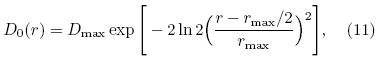
Figure 1 shows the simulated radar radial profilesof ZH, ZDR, ΦDP, and KDP. The two symmetrical raincells are clearly evident in the profiles. As a result ofattenuation, the radial profile of ZH is not symmetricto the center of the two convective cells. ZH valuesbehind the centers are obviously smaller than thosein front. The profile of ZDR reveals a similar behavior, for the same reason. However, ΦDP is immuneto attenuation and the profile of ΦDP increases monotonicallyfrom zero to 83.35◦. The KDP curve derivedfrom ΦDP shows symmetrical features for the two cells and changes from 0.07◦ to 0.45◦ km−1, with similarfluctuations in ZH and ZDR.
 |
| Fig. 1. The simulated radar radial profiles of ZH, ZDR, ΦDP, and KDP. |
In order to simulate a measured ΦDP profile, white noise with a signal to noise ratio(SNR)of 25dB was added. Figure 2 shows the noisy ΦDP profile and the de-noised profiles with mean filters(window widths of 7 and 13 points, respectively), median(7 and 13 points, respectively), FIR, Kalman, and waveletmethods. The curves de-noised by the complicate FIR, Kalman, and wavelet methods are obviously smootherthan those by the traditional mean and median methods.Namely, the FIR, Kalman, and wavelet methodshave better de-noised effects than do traditional methods.
 |
| Fig. 2. The noisy ΦDP profile(a) and the de-noised profiles by(b) and (c)7- and 13-point mean, (d) and (e)7- and 13-point median, (f)FIR, (g)Kalman, and (h)wavelet filters, respectively. |
Using the least squares fitting method, KDP isestimated with 13 consecutive ΦDP in Fig. 2. Thecorresponding KDP profiles are displayed in Fig. 3.Due to the noise and the various de-noised methods, the profiles of KDP fluctuate to varying degrees. Themaximum bias of KDP is 0.57◦ km−1 for the procedurewithout any de-noising(Fig. 3a). After de-noising, themaximum bias of KDP(Figs. 3b–h)is 0.44, 0.38, 0.46, 0.25, 0.20, 0.14, and 0.06◦ km−1, respectively. Theprofiles of KDP filtered by FIR, Kalman, and waveletmethods(Figs. 3g–h)are also found more similar tothe true KDP(Fig. 1)than the profiles filtered by thetraditional methods(Figs. 3b–e). In particular, thewavelet method in Fig. 3h proves the most similar.
 |
| Fig. 3. The KDP profile of(a)without de-noising, and with(b)7- and (c)13-point mean, (d)7- and (e)13-pointmedian, (f)FIR, (g)Kalman, and (h)wavelet filters. |
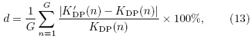
In order to quantitatively evaluate the ΦDP denoisingeffect on the KDP estimate, the mean absoluteerror ε and mean relative bias d are defined as
where K'DP and KDP represent the fitting values inFig. 2 and the simulated value in Fig. 1, respectively, n is the gate ordinal number, and G is 287, the totalnumber of fitted KDP, i.e., the total ΦDP gate numberof 300 minus a fitting width of 13.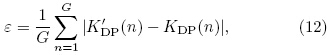
The KDP mean absolute error and mean relativebias results are listed in Table 3. Without de-noising, ε(0.19) and d(78.40%)are the largest among thoselisted in Table 3, indicating that all the methods selectedin this study de-noise KDP and more closelyrepresent the simulated KDP. The mean and medianfilters with more window points are an improvement, compared to those with fewer points. However, thisdoes not suggest that the more points the better. Thenumber of points of a window needs to be carefully selectedbased on the balance between smoothness and feature maintenance. The variables ε and d of FIR, Kalman, and wavelet methods are smaller than thosegenerated by the traditional methods, with the errorfrom the wavelet method the smallest.

The following representative real ΦDP radial profileat 0.5◦ elevation and 62.0◦ azimuth was detectedwith the mobile C-b and dual polarimetric weatherradar(POLC), which transmitted and received horizontal and vertical polarization signals simultaneously, at 0804 BT(Beijing Time)25 June 2013 in Dingyuan, Anhui Province. The main characteristics of the radar, which operated at a frequency of 5.43 GHz and a 150-m gate width, are summarized in Table 4.
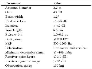
Figure 4 shows the profiles of raw data and denoisedΦDP data from the previously mentioned methods.The corresponding KDP are displayed in Fig. 5. Note that the scale of y-axis in Fig. 5a is 10 timeslarger than in Figs. 5b–h. Hence, the KDP errorsare very large if ΦDP data are not preprocessed beforeKDP fitting. KDP derived by the Kalman method(Fig. 5g)is smoother than by other methods, whichimplies that more detailed spatial features may be lostby the de-noise procedure. The FIR method(Fig. 5f)exhibits an evident boundary effect, which will influencethe KDP values at the echo boundaries. In addition, the traditional mean and median methods areless smooth. The wavelet analysis, on the other h and , is sufficiently smooth, and at the same time preservesenough detail information of weather echo, which helps effectively locate the strong convection and precipitation.Figure 6 is the corresponding plan position indicators(PPIs)of ZH and ΦDP, and Fig. 7 is the KDPPPIs corresponding to Fig. 4. KDP noise in Fig. 7ais decreased by the ΦDP de-noising(Figs. 7b–h). TheKDP PPIs of traditional mean and median methods(Figs. 7b–e)barely differ from the visual views. TheFIR, Kalman, and wavelet methods(Figs. 7f–h)arerelatively smooth compared to the traditional methods, yet the Kalman method(Fig. 7g)is too smoothfor KDP to locate the strong echoes that are easilyseen in ZH(Fig. 6a) and other KDP PPIs. For example, in Fig. 4, the average reflectivity is 42.15 dBZ inthe strong echo area from gates 183 to 352, and theaverage value 1.17◦ km−1 of KDP using the Kalmanmethod is the smallest(Table 5).
 |
| Fig. 4. As in Fig. 2, but for raw ΦDP data at 0.5◦ elevation and 62.0◦ azimuth detected at 0804 BT 25 June 2013 inDingyuan, Anhui Province. |
 |
| Fig. 5. As in Fig. 3, but the KDP profiles were obtained by using the ΦDP data in Fig. 4. Note that the scale of y-axis in(a)is 10 times larger than others. |
 |
| Fig. 6.(a)ZH(dBZ) and (b)ΦDP/sub<(deg)PPIs observed at 0.5◦ elevation and 62.0◦ azimuth detected at 0804 BT 25 June 2013 in Dingyuan, Anhui Province. The red line denotes location of the radial profile in Fig. 4. Range rings are 30-km apart. |
 |
| Fig. 7. KDP PPIs fitted by(a)raw ΦDP in Fig. 6b, and (b–h)de-noised ΦDP. |
 |
In order to further verify the influence on KDPbasedrainfall estimation, three large-scale rainfall processesduring 0200–0800 BT 25 June, 0900–1700 BT 5 July, and 0900–1700 BT 7 July 2013 are analyzed, and their ΦDP values are de-noised with various methods.The hourly rainfall is measured by 160 raingauges around the radar within 70 km. ZH is preprocessedby attenuation correction(Hu et al., 2012), and the ZH-based QPE equation is taken as
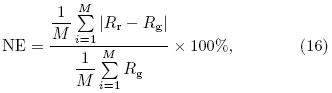
and the KDP-based QPE equation is(Liu et al., 2002):In order to analyze the accuracy of QPE, the normalizederror(NE)is defined aswhere Rr and Rg represent radar estimated and gaugemeasured rainfall, respectively, and M represents thenumber of qualified data pairs when both the estimated and measured rainfall are larger than 0.0 mm.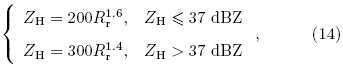

The normalized errors(NEs)of R(ZH) and R(KDP)are listed in Table 6, in which <Rg> representsthe average rainfall measured with all gauges, and the bold numbers indicate the minimum NE ofR(KDP)with different de-noising methods. As expectedR(ZH)is the best estimator when all data pairsare statistically counted, regardless of rainfall intensity(Hu et al., 2010, 2012). When only Rg values greaterthan 5, 10, 15 mm h−1 are considered, the advantage ofKDP-based estimation is evident: the heavier the precipitation, the higher the accuracy of KDP-based QPE.The SNR of the echo signal increases with greater rainfall, and the quality of the KDP data improves rapidly.Even without any pretreatment, the KDP-based estimateshave improved 10.61%(49.09% minus 38.48%) and 19.85%(51.88% minus 32.03%), in comparison toZH-based methods, when the average rainfall is heavierthan 10 and 15 mm h−1 in Table 6, respectively.In Table 6, the wavelet method is the best of these denoisingmethods. When the average rainfall is largerthan 5 mm h−1, after de-noising, the NE of R(KDP)decreases from 55.41%(raw KDP-based estimates)toa minimum of 36.30%(Kalman method), i.e., the NEof R(KDP)has improved from –7.43% to 11.68% ofR(ZH). In addition, the filter window widths, i.e., 7or 13 points of ΦDP, of traditional mean and medianfilters seem to have little influence on the results ofKDP-based QPE in all three cases.6. Discussion and summary
Since the polarimetric variable is one order ofmagnitude smaller than those measured from a polarizationdirection, they are easily influenced by noise.This is particularly the case in low SNR conditions forwhich the useful echo information is always submergedin noise. As KDP is one of the polarization parameters, how ΦDP measurements are processed and obtainingbetter KDP will directly influence the accuracyof KDP-based QPE. In recent decades, many types ofΦDP preprocessing methods have been employed; however, the specific effects of these de-noising methods and KDP-based QPE are yet to undergo comprehensivecomparative analysis.
In this paper, the ΦDP filtering effect with variouscommon methods is assessed and compared byusing numerical simulation, and finally demonstratedby real ΦDP radial. The KDP-based rainfall estimatesare also evaluated by refitting KDP to further analyzethe influence of the different ΦDP de-noising methods.
ΦDP de-noising clearly reduced the errors ofR(KDP), with the improvement more obvious whenΦDP de-noising used the more complicated Kalman, FIR, and wavelet methods, and the rainfalls were heavierthan 5 mm h−1. However, for heavier precipitation(R > 10 mm h−1), with an increased SNR, thedifferences between these methods are not significant.Therefore, for strong precipitation, the filteringmethod is not the primary consideration. Since the efficiencyof the complicated Kalman, FIR, and waveletmethods is significantly lower than that of the traditionalmethods for different precipitation types and rain rates, an efficient ΦDP de-noising program needsto be deliberately designed. For instance, the thresholdvalue of average ZH in a radial can be set todetermine whether the radial data are de-noised withfast traditional methods or more complicated ones.
In addition, it is found that the filter windowwidth of traditional filters on ΦDP had less impacton KDP-based QPE in the three large-scale rainfallprocesses. In other words, if the rain rate is greaterthan 10 mm h−1, these de-noising methods are basicallysimilar. Overall, the performance of the waveletmethod is better than other methods. Nonetheless, these results need to be appropriately verified withmore observational data, especially for convectivecloud rainfall processes.
It has been found that the value of KDP is less representativethan those of ZH and ZDR, as KDP is fittedby a number of gates over a gauge, and ZH and ZDRare detected only over a gate width. As such, the accuracyof ZH- and ZDR-based rainfall estimations shouldbe higher than the KDP-based estimation. Aside fromthe algorithm and radar system errors, precipitation isa complex dynamic, thermodynamic, and microphysicalprocess. Due to the air flow, time and space areneeded before the echoes detected by radar are transformedinto rainfall measured with ground gauges.The results in this paper further suggest that the accuracyof KDP-based rainfall estimation is higher thanthe ZH-based estimation for heavy rainfall(R > 10mm h−1), and that after ΦDP de-noising, the accuracyof KDP-based QPE is more accurate than ZH-basedQPE, even for light to moderate rain(R >5 mm h−1).
| Brandes, E. A., G. Zhang, and J. Vivekanandan, 2003: An evaluation of a drop distribution-based polari-metric radar rainfall estimator. J. Appl. Meteor., 42, 652-660. |
| Bringi, V. N., and V. Chandrasekar, 2001: Polarimetric Doppler Weather Radar: Principles and Applica-tions. Cambridge University Press, Cambridge, 635 pp. |
| Carey, L. D., S. A. Rutledge, D. A. Ahijevych, et al., 2000: Correcting propagation effects in C-band po-larimetric radar observations of tropical convection using differential propagation phase. J. Appl. Me-teor., 39, 1405-1433. |
| Chandrasekar, V., V. N. Bringi, N. Balakrishnan, et al., 1990: Error structure of multi-parameter radar and surface measurements of rainfall. Part III: Specific differential phase. J. Atmos. Oceanic Technol., 7, 621-629. |
| Cifelli, R., V. Chandrasekar, S. Lim, et al., 2011: A new dual-polarization radar rainfall algorithm: Appli-cation in Colorado precipitation events. J. Atmos. Oceanic Technol., 28, 352-364. |
| Giangrande, S. E., R. McGraw, and L. Lei, 2013: An application of linear programming to polarimet-ric radar differential phase processing. J. Atmos. Oceanic Technol., 30, 1716-1729. |
| Gorgucci, E., G. Scarchilli, and V. Chandrasekar, 1999: Specific differential phase estimation in the presence of nonuniform rainfall medium along the path. J. Atmos. Oceanic Technol., 16, 1690-1697. |
| Gorgucci, E., G. Scarchilli, and V. Chandrasekar, 2000: Practical aspects of radar rainfall estimation using specific differential propagation phase. J. Appl. Me-teor., 39, 945-955. |
| Grazioli, J., M. Schneebeli, and A. Berne, 2014: Accu-racy of phase-based algorithms for the estimation of the specific differential phase shift using simu-lated polarimetric weather radar data. IEEE Trans. Geosci. Remote Sens., 11, 763-767. |
| He Yuxiang, Lü Daren, Xiao Hui, et al., 2009: Atten-uation correction of reflectivity for X-band dual polarization radar. Chinese J. Atmos. Sci., 33, 1027-1037. (in Chinese) |
| Hu Zhiqun, Liu Liping, Chu Rongzhong, et al., 2010: Study of different attenuation correction methods in association with rainfall estimation for X-band po-larimetric radars. Acta Meteor. Sinica, 24, 602-613. |
| Hu Zhiqun, Liu Liping, and Wang Lirong, 2012: A quality assurance procedure and evaluation of rainfall esti-mates for C-band polarimetric radar. Adv. Atmos. Sci., 29, 144-156. |
| Hu Zhiqun and Liu Liping, 2014: Applications of wavelet analysis in differential propagation phase shift data de-noising. Adv. Atmos. Sci., 31, 825-835. |
| Hubbert, J. V., V. Chandrasekar, V. N. Bringi, et al., 1993: Processing and interpretation of coher-ent dual-polarized radar measurements. J. Atmos. Oceanic Technol., 10, 155-164. |
| Hubbert, J. V., and V. N. Bringi, 1995: An iterative filter-ing technique for the analysis of copolar differential phase and dual-frequency radar measurements. J. Atmos. Oceanic Technol., 12, 643-648. |
| Jameson, A. R., 1991: Polarization radar measurements in rain at 5 and 9 GHz. J. Appl. Meteor., 30, 1500- 1513. |
| Krajewski, W. F., G. Villarini, and J. A. Smith, 2010: Radar-rainfall uncertainties. Bull. Amer. Meteor. Soc., 91, 87-94. |
| Liu Liping, Xu Baoxiang, and Cai Qiming, 1989: The effects of attenuation by precipitation and sampling error on measuring accuracy of 713 type dual linear polarization radar. Plateau Meteorology, 8, 181-188. (in Chinese) |
| Liu Liping, Ge Renshen, and Zhang Peiyuan, 2002: A study of method and accuracy of rainfall rate and liquid water content measurements by dual linear polarization Doppler radar. Chinese J. Atmos. Sci., 26, 709-720. (in Chinese) |
| Liu, L. P., G. L. Wang, Z. Q. Hu, et al., 2013: Multi-ple Radar Integration Technology and Application to Heavy Rainfall Monitoring in Southern China. China Meteorological Press, Beijing, 92-104. (in Chinese) |
| May, P., T. D. Keecnan, D. Zrnic, et al., 1999: Polari-metric radar measurements of tropical rain at 5-cm wavelength. J. Appl. Meteor., 38, 750-765. |
| Melnikov, V. M., D. S. Zrnic, R. J. Doviak, et al., 2003: Calibration and Performance Analysis Of NSSL's Polarimetric WSR-88D. NOAA/NSSL Rep., 77 pp. |
| Proakis, J. G., and D. G. Manolakis, 1988: Introduction to Digital Signal Processing. Macmillan Publishing Co., 944 pp. |
| Ryzhkov, A. V., and D. S. Zrnić, 1995: Comparison of dual-polarization radar estimators of rain. J. At-mos. Oceanic Technol., 12, 249-256. |
| Ryzhkov, A. V., and D. S. Zrnić, 1996: Assessment of rainfall measurement that uses specific differential phase. J. Appl. Meteor., 35, 2080-2090. |
| Ryzhkov, A. V., S. E. Giangrande, and T. J. Schuur, 2005: Rainfall estimation with a polarimetric prototype of the WSR-88D. J. Appl. Meteor., 44, 502-515. |
| Sachidananda, M., and D. S. Zrnic, 1987: Rain rate esti-mates from differential polarization measurements. J. Atmos. Oceanic Technol., 4, 588-598. |
| Scarchilli, G., E. Gorgucci, V. Chandrasekar, et al., 1993: Rainfall estimating using polarimetric technique at C-band frequencies. J. Appl. Meteor., 32, 1150- 1160. |
| Schneebeli, M., and A. Berne, 2012: An extended Kalman filter framework for polarimetric X-band weather radar data processing. J. Atmos. Oceanic Technol., 29, 711-730. |
| Ulbrich, C. W., 1983: Natural variations in the analyti-cal form of the raindrop size distribution. J. Appl. Meteor., 22, 1764-1775. |
| Vulpiani, G., M. Montopoli, L. D. Passeri, et al., 2012: On the use of dual-polarized C-band radar for op-erational rainfall retrieval in mountainous areas. J. Appl. Meteor. Climatol., 51, 405-425. |
| Wang, Y., and V. Chandrasekar, 2009: Algorithm for es-timation of the specific differential phase. J. Atmos. Oceanic Technol., 26, 2565-2578. |
| Wilson, J. W., and E. A. Brandes, 1979: Radar measure-ment of rainfall—A summary. Bull. Amer. Meteor. Soc., 60, 1048-1058. |
| Zrnic, D., and A. Ryzhkov, 1996: Advantages of rain measurements using specific differential phase. J. Atmos. Oceanic Technol., 13, 454-464. |