 2015,vol.29
The Chinese Meteorological Society
Article Information
- Li Ruiqing, LÜ Shihua, Han Bo, GAO Yanhong, 2015
- Connections between the South Asian summer monsoon and the tropical sea surface temperature in CMIP5
- J. Meteor. Res., 29(1): 106-118
- http://dx.doi.org/10.1007/s13351-014-4031-5.
Article History
- Received February 26, 2014;
- in final form August 31, 2014


2 University of Chinese Academy of Sciences, Beijing100049(Received February 26, 2014; in final form August 31, 2014)
The South Asian Summer Monsoon(SASM)isa major component of the Asian–Australian monsoon system. It dominates the rainfall distribution over South Asia and has important economic and social effects(Wu et al., 2009). Its intensityis indicated by the all-India monsoon rainfall index(AIMRI)(Parthasarathy et al., 1991),which represents the area-weighted seasonal average(June–September,JJAS)rainfall over continental India(Parthasarathy et al., 1991). Besides seasonal variation,the AIMRI usually exhibits significant variabilityon subseasonal and interannual timescales(Webster and Tomas, 1998; Annamalai et al., 1999).
Since the seminal work of Walker and Bliss(1932),the simultaneous sea surface temperature anomalies(SSTAs)associated with El Niño in the central–eastern Pacific have been found associated with forcing the interannual variability of the AIMRI(Ju and Slingo, 1995; Chang et al., 2000). Many studieshave depicted the importance of central–eastern Pacific SSTAs on global climate(Sikka,1980; Rasmusson and Carpenter, 1983; Nigam,1994; Meehl et al., 2000; Slingo and Annamalai, 2000; Annamalai and Liu, 2005). Generally,precipitation in India decreaseswhen an El Ni˜no event occurs(Webster and Tomas, 1998). The connection between the SASM and SSTAsmay provide a reference to predictions of the interannual fluctuations of SASM(Charney and Shukla, 1981), and how such a relationship is represented in climate models has also been discussed(Li et al., 2013).
Since the 1980s,the El Ni˜no–monsoon connectionhas been reported to have weakened relative to previous decades,especially in the 1990s(Kinter et al., 2002). Some have attributed this to global warming(Kumar et al., 1999),while others have proposed thatthe link between monsoon and SST varies on a decadaltimescale(Parthasarathy et al., 1991). Recently,thedeficits of the AIMRI in 2002 and 2004(19% and 13% below normal,respectively),both accompanyingmoderate El Ni˜no events,suggested that the El Ni˜no–monsoon connection has become stronger again. Astrong connection between El Niño and SASM benefits the prediction of the latter,as prediction of theformer up to one year in advance has progressed inrecent years(Latif et al., 1998).
The effect of global warming on the El Ni˜no–monsoon relationship remains uncertain. Some reported that climate change has little impact on SASM(Mahfouf et al., 1994; Timbal et al., 1995),while others found increased monsoon rainfall compared to thepre-industrial period(Meehl and Washington, 1993;Hu et al., 2000; May,2002; Meehl and Arblaster, 2003). Moreover,the robustness of the El Niño–monsoon relationship is not consistent among thesestudies. The uncertainty of the El Niño–monsoon relationship under global warming has been studied bybyAshrit et al.(2001,2003,2005). They first reportedno “systematic change”(Ashrit et al., 2003),but latersuggested that the relationship would be no longer significant after 2050(Ashrit et al., 2005).
Analysis of the historical and projected variationsin the El Niño–monsoon coupling has been carried outwith different global coupled models in the Intergovernmental Panel on Climate Change(IPCC)FourthAssessment Report(AR4). Compared to previousgenerations of models,the AR4 models more accurately represent El Niño events(AchutaRao and Sperber, 2006; Guilyardi,2006; Joseph and Nigam, 2006).Importantly,Turner et al.(2005)demonstrated animprovement in reproducing the tropical Pacific meanstate through the use of flux adjustment.
The Coupled Model Intercomparison Projectphase 5(CMIP5)has provided further improved models in simulating historical and future climate and predicting the change in the relationship between El Ni˜no and the monsoon. In this study,we assess the abilityof these models in reproducing the features of SASM,El Ni˜no, and their connections. 2. Models and observations
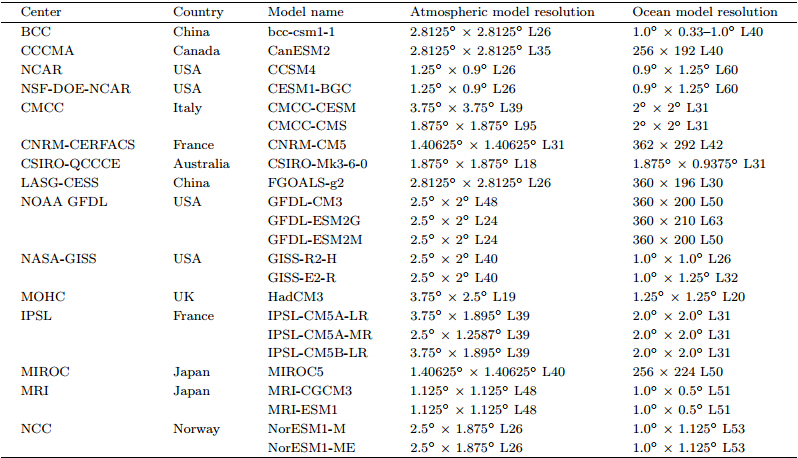
Table 1 provides the basic details of the 23 CMIP5model configurations used in this study. Detailed descriptions of the models and experiments in CMIP5 areavailable at http://cmip-pcmdi.llnl.gov/cmip5/. Forconvenience,all the simulation results are regriddedto 1°×1°data by using a bilinear interpolation algorithm.
The observed precipitation is represented by thedata from the Climate Prediction Center MergedAnalysis of Precipitation(CMAP)(Xie and Arkin, 1996). The AIMRI offered by the Indian Instituteof Tropical Meteorology(www.tropmet.res.in)is used.SST data are from the Hadley Centre Sea Ice and SSTdataset(Rayner et al., 2003). The velocity potentialat 200 hPa is derived from the NCEP/NCAR reanalysis dataset(Kalnay et al., 1996). For historical simulations,the study period is from January 1979 toDecember 2005.
precipitationOver the Asian summer monsoon region,theobserved precipitation in the rainy season(JJAS)(Fig. 1a)indicates three intense precipitation centers:(1)the one in the Indian summer monsoon region(5°–30°N,65°–95°E),which can be evaluated bythe AIMRI;(2)the one in the western North Pacific monsoon region(10°–20°N,110°–150°E); and (3)the one in the eastern equatorial Indian Ocean region(10°S–0°,90°–110°E),where the interannual variability of precipitation is also strong. These centers respond differently to El Niño forcing, and modulate oneanother(Annamalai and Liu, 2005; Annamalai and Sperber, 2005).
From the multi-model ensemble results(Fig. 1b),the climatological mean for 1979–2005 precipitationin JJAS is similar to the observations,but the st and ard deviation values are much weaker,because of thecancellation among all models during ensemble averaging. The multi-model ensemble mean captured wellthe detailed structure in precipitation over India,inparticular the strong rainfall along the west coast and over the Bay of Bengal.
 |
| Fig. 1. Seasonal mean(JJAS)precipitation climatology(shaded; mm day-1) and st and ard deviation(dashed contour;mm day-1)of(a)observation and (b)the ensemble mean of the CMIP5 models in the period 1979–2005,with contourintervals of 1.0 and 0.2 mm day-1,respectively. |
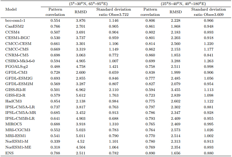
Table 2 gives the root-mean-square differences(RMSDs),the ratio of the st and ardized variances(STDRs)relative to the observation, and the pattern correlations of climatological mean precipitationbetween the simulation and observation in the monsoon domain(25°S–40°N,40°–180°E). The results ofmost models are similar to the observations,except forGISS-E2-H. Most models in CMIP5 reproduce wellthe climatological mean precipitation of the SASM,with greater pattern correlations and smaller RMSDs.The pattern correlation for the multi-model ensemblemean is 0.89 and its RMSD is 1.66.
Concentrating solely on the Indian region(5°–30°N,65°–95°E),the results are displayed as a Taylordiagram(Fig. 2). There are large differences in thesummer precipitation(JJAS)pattern correlation between individual model and observation. The patterncorrelations from CanESM2,GFDL-CM3,HadCM3, and IPSL-CM5A-LR are greater than those from othermodels. The pattern correlation for the multi-modelensemble mean result is 0.788 and its RMSD is 2.51.Therefore,compared with the monsoon domain,although the pattern correlation is smaller and theRMSD is greater,most models in CMIP5 reproducewell the climatological mean precipitation over theSASM region.
 |
|
 |
| Fig. 2.Taylor diagram of the precipitation over the Indian monsoon region(5°–30°N,65°–95°E)for the 23 models and their ensemble mean compared to the observation. |
The climatological mean annual cycle of SASMprecipitation over the region(5°–30°N,65°–95°E)from 1979 to 2005 is given in Fig. 3a. The observed strongest SASM precipitation of about 8.19 mmday-1occurs in July. Compared to observations,although most models show similar peak precipitationin July,the intensity of the precipitation during JJASis underestimated,with the precipitation in July fromthe multi-model ensemble mean being only 7.15 mmday-1. Moreover,the simulated main rainfall periodlags the observation by one month. The differences inthe climatological mean annual precipitation betweenthe models and observation are shown in Fig. 3b. Themaximum difference of about 2.90 mm day-1appearsin June for the multi-model ensemble mean result.
 |
| Fig. 3.The annual cycle of(a)precipitation(mm day-1)during 1979–2005 over the Indian monsoon region(5°–30°N,65°–95°E) and (b)the differences between the models and observation. |
An El Ni˜no event occurs when the normalizedmean SSTA during JJAS averaged over the Ni˜no3.4region(5°S–5°N,120°–170°W)is greater than 1. TheEl Ni˜no event usually maintains until the followingyear(Annamalai et al., 2007). Figure 4 shows thecomposite evolution of Niño3.4 SSTAs during an ElNi˜no event from all the models and their ensemblemean. The SSTA evolution from most of the modelsquite closely matches the observation,as does their ensemble mean. Most models have an SSTA peak closeto(or in)December in an El Niño year,whereas theobserved peak mainly occurs in October. However,there are some exceptions. For example,the SSTAs inCSIRO-Mk3-6-0 and MIROC5 have no peaks throughout the entire boreal winter during the El Niño event.
 |
| Fig. 4.Monthly temporal evolution of the composite SST anomalies(in st and ard deviations;℃)averaged over theNi˜no3.4 region(5°S–5°N,120°–170°W)for different coupled models in the historical simulations. The composites arebased on strong El Ni˜no events(>1.0 st and ard deviations of SST anomalies over the Niño3.4 region during JJAS). Years0 and 1 correspond to the typical life cycle of El Niño in which it peaks around December at the end of year 0. |
The spatiotemporal evolution of SSTAs along theequatorial Pacific in an El Niño event is given in Fig. 5. The intensification of the warm SSTA in the central eastern Pacific is significant(Fig. 5a),especiallyduring the summer monsoon season(indicated by thetwo horizontal dotted lines in Fig. 5). Such a feature is well represented by the multi-model ensemblemean,although the magnitude of the simulated SSTAis much smaller.
 |
| Fig. 5.Evolution of monthly SSTAs(℃)in the equatorial(5°S–5°N)Pacific during El Ni˜no years from(a)observation and (b)ensemble mean of CMIP5 models. The horizontal dashed lines represent the duration of the summermonsoon season. The time coordinate starts with Januaryof year 0 of the developing phase of an El Niño event and ends with December of year 1 of the decaying phase ofthe El Niño event. The composites are based on strong ElNi˜no events(>1.0 st and ard deviations of SST anomaliesover the Niño3.4 region during JJAS) |
The spatial distribution of composite SSTAs inEl Ni˜no years is shown in Fig. 6. The SSTA variation characteristics of the multi-model ensemble meanresult are similar to the observation: there are positive SSTAs over the eastern equatorial Pacific and the Arabian Sea, and negative SSTAs are mainly located in Northwest Pacific and the maritime continent. The strengths of the simulated SSTAs fromthe multi-model ensemble mean are weaker than observed,especially in the eastern equatorial Pacific and Northwest Pacific.
 |
| Fig. 6.Seasonal mean(JJAS)SSTA(℃)during El Ni˜ no years from(a)observation and (b)ensemble mean of CMIP5models. The composites are based on strong El Ni˜no events(>1.0 st and ard deviations of SST anomalies over theNi˜no3.4 region during June–September). Positive values are shaded progressively,while negative values are shown asdashed contours with an interval of 0.4℃ |
When an El Niño event develops,significant and positive SSTAs in central and eastern equatorial Pacific induce intensified convection in central Pacific and suppressed convection over the maritime continent. This feature is captured well by the multi-modelensemble mean,but the magnitude of the simulatedanomalies of precipitation and SSTAs are both weakerthan in the observation(Fig. 7). From the compositeprecipitation in El Ni˜no years,the precipitation variation characteristics are similar to the observation inthe Indian monsoon region,the maritime continent, and the western equatorial Pacific. In contrast,thenegative precipitation anomalies over the South ChinaSea and Philippine Sea are not reproduced well bymost models(Fig. 8).
 |
| Fig. 7.As in Fig. 5,but for precipitation anomalies(mm day-1)from(a)observation and (b)ensemble meanof CMIP5 models. Positive values are shaded progressively,while negative values are shown in contours with an interval of 1.0 mm day-1in(a) and 0.5 mm day-1in(b). |
 |
| Fig. 8. Seasonal mean(JJAS)precipitation(mm day-1)anomalies during El Ni˜ no years from(a)observation and (b)ensemble mean of CMIP5 models. The composites are based on strong El Ni˜ no events(>1.0 st and ard deviations ofSST anomalies over the Ni˜no3.4 region during JJAS). Negative values are shaded progressively,while positive values areshown as dashed contours with an interval of 1.0 mm day-1.. |
Tropical SSTAs impact the global precipitationthrough affecting large-scale atmospheric circulations.During El Ni˜no years,latent heat sources redistribute, and latent heat sinks in the equatorial Pacific determine the descending and rising branches of the Walkercell. This is possibly the most important mechanismfor the El Niño–monsoon teleconnection(Charney and Shukla, 1981; Parthasarathy et al., 1991; Latif et al., 1998; Kinter et al., 2002). The velocity potentialanomaly at 200 hPa during El Niño events is givenin Fig. 9. The multi-model ensemble mean gives asimilar spatial distribution pattern of the velocity potential anomalies at 200 hPa as the reanalysis,but underestimates the magnitude, and wrongly locates thecenter too far east.
 |
| Fig. 9.As in Fig. 8,but for the anomalous velocity potential(106 m2s-1)at 200 hPa from(a)observation and (b)ensemble mean of CMIP5 models. Negative values are shaded progressively,while positive values are shown as solidcontours with an interval of 106m2s-1. |
Therefore,although the magnitude of the ElNi˜no-induced signals is underestimated,the development of SSTAs,the eastward movement of the precipitation anomaly, and the distribution of the velocitypotential anomaly in tropical zones are all capturedwell by most CMIP5 models. These results representan improvement over those from CMIP3; for instance,Annamalai et al.(2007)reported a large diversityin both the amplitude and spatial pattern of SSTAs and precipitation anomalies over the tropical Pacificin CMIP3(see Figs. 2–5 of their paper).3.3.2 Correlation between AIMRI and SSTAs
The AIMRI was first defined by AchutaRao and Sperber(2002)by calculating the area-weighted rainfall over continental India during JJAS. It is usuallyused to represent the intensity of SASM. The AIMRIdata based on observed precipitation are used in thisstudy. We also calculate the AIMRI by using CMAPdata, and find little difference from the observed values. To calculate the simulated AIMRI in differentclimate models,the gridded data on the l and over theregion(5°–30°N,65°–95°E)are used.
The correlation coefficient between SSTAs and AIMRI is given in Fig. 10. The observation results(Fig. 10a)display that when the AIMRI is strongerthan normal,there are a statistically significant negative SSTA in the eastern equatorial Pacific and apositive SSTA in the western equatorial Pacific and the maritime continent. Such features are reproducedwell by the ensemble mean of the CMIP5 models(Fig. 10b). The correlation coefficient from most models isnegative in the central eastern Pacific and positive inthe maritime continent. However,most models tendto overestimate the positive correlations over the maritime continent and in Northwest Pacific. This may becaused by the coupled models overestimating the extent of the positive SSTA during El Niño events alongthe western equatorial Pacific(Fig. 5; AchutaRao and Sperber, 2006; Joseph and Nigam, 2006).
 |
| Fig. 10. Correlation patterns between the seasonal mean(JJAS)AIMRI and SSTAs from(a)observation and (b)ensemble mean of CMIP5 models from 1979 to 2005. Only the correlations statistically significant at the 95% level aremarked. Negative(positive)values are shown as dashed(solid)contours with an interval of 0.2.. |
The correlation patterns between AIMRI and SSTAs in both historical simulations(1979–2005) and future projections(2070–2096)under two representative concentration pathway(RCP)scenarios(RCP4.5 and RCP8.5)are shown in Fig. 11. Based on the previous discussion,the most significant correlation between AIMRI and SSTAs usually appears in the eastern equatorial Pacific. Comparing the result from thehistorical simulations with that from the projectionunder RCP8.5 finds that most models exhibit a negative correlation between AIMRI and SSTAs in theeastern equatorial Pacific and the negative correlation indeed becomes weaker,or even reversed. Sucha result is especially significant in the multi-modelensemble mean. An intensified negative correlationis only given by CanESM2 and IPSL-CM5A-LR. ForRCP4.5,meanwhile,the correlation between AIMRI and SSTAs shows different changes for different models. The results from bcc-csm1-1,CCSM4,CESM1-BGC,GFDL-CM3, and IPSL-CM5A-MR show a significantly weakened correlation between SSTAs and AIMRI in the eastern equatorial Pacific,while the restof the models tend to show either an inverse changeor little change. Therefore,from the projections givenby the climate models,if the future external forcingon the climate system is as strong as that defined under RCP8.5,the negative correlation between El Ni˜no and SASM is likely to become weaker,or even positive,during 2070–2096. If the external forcing is moderate,as under RCP4.5,the change in the connection between El Niño and SASM is difficult to ascertain. Theuncertainties in the change of the El Ni˜no–monsoonrelationship under global warming are consistent withprevious research. Ashrit et al.(2005)suggested thatthe relationship will cease to be significant after 2050.
 |
| Fig. 11. Correlation patterns between the seasonal mean(JJAS)AIMRI and SSTAs from simulations of 12 CMIP5models and their ensemble means for the historical simulations from 1979 to 2005(left column),RCP4.5(middle column), and RCP8.5(right column)from 2070 to 2096. Only the correlations statistically significant at or above the 95% levelare marked. Negative(positive)values are shown as dashed(solid)contours.. |
Based on 23 climate model simulation results fromCMIP5,the South Asian summer monsoon and its relationship with SSTAs are discussed. The main conclusions are:
(1)Most coupled models accurately simulate theclimatological mean spatial pattern of monsoon precipitation. However,the main rainfall period from themulti-model ensemble mean lags that of the reanalysisby one month.
(2)Most of the models accurately represent theevolution of the SST,precipitation, and atmosphericcirculation in an El Niño event; however,the magnitudes of these signals are underestimated.
(3)For future projections,if the external forcingon the climate system is strong,as under RCP8.5,the negative correlation between an El Niño event and SASM weakens or even becomes positive in theperiod 2070–2096. However,if the external forcing ismoderate,as under RCP4.5,the change of correlationbetween El Ni˜no and SASM is difficult to ascertain.
In this study,we only examined the relationshipbetween El Ni˜no events and SASM precipitation; however,other factors such as the Himalayan snow,mayalso potentially affect SASM precipitation,as reportedby Kripalani and Kulkarni(1999). Using Soviet snowdepth data,they found that the winter snow depthover western Eurasia is negatively correlated withSASM precipitation, and positively correlated withsnow depth over eastern Eurasia. Droughts unrelatedto El Niño events may be related to snow depth inthe previous winter over western Eurasia(Kripalani and Kulkarni, 1999). Since such a dipole snow configuration has also been noted in CMIP3(IPCC,2007;Kripalani et al., 2007a,b),further diagnostic work onthe relationship between snow and SASM in CMIP5is clearly required.
| [1] | AchutaRao, K., and K. R. Sperber, 2002: Simulation of the El Niño Southern Oscillation: Results from the coupled model intercomparison project. Climate Dyn., 19, 191-209, doi: 10.1007/s00382-001-0221-9. |
| [2] | AchutaRao, K., and K. R. Sperber, 2006: ENSO simulation in coupled ocean-atmosphere models: Are the current models better? Climate Dyn. , 27, 1-15, doi:10.1007/s00382-006-0119-7. |
| [3] | Annamalai, H., J. M. Slingo, K. R. Sperber, et al., 1999: The mean evolution and variability of the Asian summer monsoon: Comparison of ECMWF and NCEP-NCAR reanalyses. Mon. Wea. Rev., 127, 1157-1186, doi: 10.1175/1520-0493(1999)127<1157:TMEAVO>2.0.CO;2. |
| [4] | Annamalai, H., and K. R. Sperber, 2005: Regional heat sources and the active and break phases of boreal summer intraseasonal (30-50 day) variability. J. At-mos. Sci., 62, 2726-2748, doi: 10.1175/JAS3504.1. |
| [5] | Annamalai, H., and P. Liu, 2005: Response of the Asian summer monsoon to changes in El Niño properties. Quart. J. Roy. Meteor. Soc., 131, 805-831, doi:10.1256/qj.04.08. |
| [6] | Annamalai, H., K. Hamilton, and K. R. Sperber, 2007: The South Asian summer monsoon and its relation-ship with ENSO in the IPCC AR4 simulations. J. Climate, 20, 1071-1092, doi: 10.1175/JCLI4035.1. |
| [7] | Ashrit, R. G., K. R. Kumar, and K. K. Kumar, 2001: ENSO-monsoon relationships in a greenhouse warm-ing scenario. Geophys. Res. Lett., 28, 1727-1730, doi: 10.1029/2000GL012489. |
| [8] | Ashrit, R. G., H. Douville, and K. R. Kumar, 2003: Re-sponse of the Indian monsoon and ENSO-monsoon teleconnection to enhanced greenhouse effect in the CNRM coupled model. J. Meteor. Soc. Japan, 81, 779-803, doi: 10.2151/jmsj.81.779. |
| [9] | Ashrit, R. G., A. Kitoh, and S. Yukimoto, 2005: Tran-sient response of ENSO-monsoon teleconnection in MRI-CGCM2. 2 climate change simulations. J. Me-teor. Soc. Japan, 83, 273-291, doi: 10.2151/jmsj.83.273. |
| [10] | Chang, C. P., Y. Zhang, and T. Li, 2000: Interannual and interdecadal variations of the East Asian sum-mer monsoon and tropical Pacific SSTs. Part I: Roles of the subtropical ridge. J. Climate, 13, 4310-4325, doi: 10.1175/1520-0442(2000)013013<4310:IAIVOT>2.0.CO;2. |
| [11] | Charney, J. G., and J. Shukla, 1981: Predictability of monsoons. Monsoon Dynamics, J. Lighthill and R. P. Pearce, Eds., Cambridge University Press, Cam-bridge, 99-109. |
| [12] | Guilyardi, E., 2006: El Niño-mean state-seasonal cycle interactions in a multi-model ensemble. Climate Dyn., 26, 329-348, doi: 10.1007/s00382-005-0084-6. |
| [13] | Hu, Z. Z., M. Latif, E. Roeckner, et al., 2000: Intensi-fied Asian summer monsoon and its variability in a coupled model forced by increasing greenhouse gas. Geophys. Res. Lett., 27, 2681-2684, doi: 10.1029/2000GL011550. |
| [14] | IPCC, 2007: Climate Change: The Physical Science Ba-sis Summary for Policymakers. Intergovernmental Panel on Climate Change, Geneva, Switzerland, 996 pp. |
| [15] | Joseph, R., and S. Nigam, 2006: ENSO evolution and teleconnections in IPCC's twentieth-century climate simulations: Realistic representation? J. Climate,19, 4360-4377, doi: 10.1175/JCLI3846.1. |
| [16] | Ju, J., and J. Slingo, 1995: The Asian summer monsoon and ENSO. Quart. J. Roy. Meteor. Soc., 121,1133-1168, doi: 10.1002/qj.49712152509. |
| [17] | Kalnay, E., M. Kanamitsu, R. Kistler, et al., 1996: The NCEP/NCAR 40-year reanalysis project. Bull. Amer. Meteor. Soc., 77, 437-471, doi: 10.1175/1520-0477(1996)077<0437:TNYRP>2.0.CO;2. |
| [18] | Kinter, J. L., K. Miyakoda, and S. Yang, 2002: Recent change in the connection from the Asian mon-soon to ENSO. J. Climate, 15, 1203-1215, doi:10.1175/1520-0442(2002)015<1203:rcitcf>2.0.co;2. |
| [19] | Kripalani, R. H., and A. Kulkarni, 1999: Climatology and variability of historical Soviet snow depth data: Some new perspectives in snow-Indian monsoon teleconnections. Climate Dyn., 15, 475-489, doi:10.1007/s003820050294. |
| [20] | Kripalani, R. H., J. H. Oh, and H. S. Chaudhari, 2007a: Response of the East Asian summer monsoon to dou-bled atmospheric CO2 : Coupled climate model sim-ulations and projections under IPCC AR4. Theor. Appl. Climatol., 87, 1-28, doi: 10.1007/s00704-006-0238-4. |
| [21] | Kripalani, R. H., J. H. Oh, A. Kulkarni, et al., 2007b: South Asian summer monsoon precipitation vari-ability: Coupled climate model simulations and pro-jections under IPCC AR4. Theor. Appl. Climatol., 90, 133-159, doi: 10.1007/s00704-006-0282-0. |
| [22] | Kumar, K. K., B. Rajagopalan, and M. A. Cane, 1999: On the weakening relationship between the Indian monsoon and ENSO. Science, 284, 2156-2159, doi:10.1126/science.284.5423.2156. |
| [23] | Latif, M., D. Anderson, T. Barnett, et al., 1998: A review of the predictability and prediction of ENSO. J. Geophys. Res., 103, 14375-14393, doi:10.1029/97JC03413. |
| [24] | Li Ruiqing, Lü Shihua, and Han bo, 2013: Simulations of Asian-Australian monsoon circulation and vari-ability by 10 CMIP5 models. J. Trop. Meteor., 29,749-758. (in Chinese) |
| [25] | Mahfouf, J. F., D. Cariolle, J. F. Royer, et al., 1994: Response of the Meteo-France climate model to changes in CO2 and sea surface temperature. Cli-mate Dyn., 9, 345-362, doi: 10.1007/BF00223447. |
| [26] | May, W., 2002: Simulated changes of the Indian summer monsoon under enhanced greenhouse gas conditions in a global time-slice experiment. Geophys. Res. Lett., 29, 22-1-22-4, doi: 10.1029/2001GL013808. |
| [27] | Meehl, G. A., and W. M. Washington, 1993: South Asian summer monsoon variability in a model with doubled atmospheric carbon dioxide concen-tration. Science, 260, 1101-1104, doi: 10.1126/sci-ence.260.5111.1101. |
| [28] | Meehl, G. A., G. J. Boer, C. Covey, et al., 2000: The cou-pled model intercomparison project (CMIP). Bull. Amer. Meteor. Soc., 81, 313-318, doi: 10.1175/1520-0477(2000)081<0313:TCMIPC>2.3.CO;2. |
| [29] | Meehl, G. A., and J. M. Arblaster, 2003: Mechanisms for projected future changes in South Asian mon-soon precipitation. Climate Dyn., 21, 659-675, doi:10.1007/s00382-003-0343-3. |
| [30] | Nigam, S., 1994: On the dynamical basis for the Asian summer monsoon rainfall-El Niño relation-ship. J. Climate, 7, 1750-1771, doi: 10.1175/1520-0442(1994)007<1750:OTDBFT>2.0.CO;2. |
| [31] | Parthasarathy, B., K. R. Kumar, and A. A. Munot, 1991: Evidence of secular variations in Indian monsoon rainfall-circulation relationships. J. Cli-mate, 4, 927-938, doi: 10.1175/1520-0442(1991)004<0927:EOSVII>2.0.CO;2. |
| [32] | Rasmusson, E. M., and T. H. Carpenter, 1983: The relationship between eastern equatorial Pacific sea surface temperatures and rainfall over India and Sri Lanka. Mon. Wea. Rev., 111, 517-528, doi:10.1175/1520-0493(1983)111111<0517:TRBEEP>2.0.CO;2. |
| [33] | Rayner, N. A., D. E. Parker, E. B. Horton, et al., 2003: Global analyses of sea surface temperature, sea ice, and night marine air temperature since the late nineteenth century. J. Geophys. Res., 108, 4407, doi: 10.1029/2002JD002670. |
| [34] | Sikka, D. R., 1980: Some aspects of the large scale fluc-tuations of summer monsoon rainfall over India in relation to fluctuations in the planetary and regional scale circulation parameters. Proceedings of the In-dian Academy of Sciences-Earth and Planetary Sci-ences, 89, 179-195, doi: 10.1007/BF02913749. |
| [35] | Slingo, J. M., and H. Annamalai, 2000: 1997: The El Niño of the century and the response of the In-dian summer monsoon. Mon. Wea. Rev., 128,1778-1797, doi: 10.1175/1520-0493(2000)128128<1778:TENOOT>2.0.CO;2. |
| [36] | Timbal, B., J. F. Mahfouf, J. F. Royer, et al., 1995: Sensitivity to prescribed changes in sea surface temperature and sea ice in doubled carbon diox-ide experiments. Climate Dyn., 12, 1-20, doi: 10.1007/BF00208759. |
| [37] | Turner, A. G., P. M. Inness, and J. M. Slingo, 2005: The role of the basic state in the ENSO-monsoon relationship and implications for predictability. Quart. J. Roy. Meteor. Soc., 131, 781-804, doi:10.1256/qj.04.70. |
| [38] | Walker, G. T., and E. W. Bliss, 1932: World weather. Meteor. Soc., 4, 32. |
| [39] | Wu Bo, Zhou Tianjun, Li Tim, et al., 2009: Interannual variability of the Asian-Australian monsoon and ENSO simulated by an ocean-atmosphere coupled model. Chinese J. Atmos. Sci., 33, 285-299, doi: 10.3878/j.issn.1006-9895.2009.02.08. (in Chinese) |
| [40] | Xie, P., and P. A. Arkin, 1996: Analyses of global monthly precipitation using gauge observations, satellite estimates, and numerical model predic-tions. J. Climate, 9, 840-858, doi: 10.1175/1520-0442(1996)009<0840:AOGMPU>2.0.CO;2. |
| [41] | Webster, P. J., and R. Tomas, 1998: Monsoons: Pro-cesses, predictability, and the prospects for predic-tion. J. Geophys. Res., 103, 14451-14510, doi:10.1029/97JC02719. |