 2015,vol.29
The Chinese Meteorological Society
Article Information
- HAN Bo , LÜ Shihua, GAO Yanhong, AO Yinhuan, 2015.
- Response of atmospheric energy to historical climate change in CMIP5
- J. Meteor. Res., 29(1): 093-105
- http://dx.doi.org/10.1007/s13351-014-4016-4.
Article History
- Received February 26, 2014;
- in final form August 28, 2014


Climate change in recent decades,usually represented as the increase of global surface air temperature(SAT)(Willmott and Legates, 1993; Dixon and Lanzante, 1999; Jones et al., 1999; Watterson et al., 1999; Simmons et al., 2004; Bodri and Cermak, 2005;Zhou and Yu, 2006; Meehl et al., 2007),is also calledglobal warming. Because the entire climate systemcontains several subsystems(Peixoto and Oort, 1992),there are various climate change indications,e.g.,reduction of sea-ice concentration(Ingram et al., 1989;Johannessen et al., 2004),rising sea levels(Meehl et al., 2005; Church and White, 2006),rainforest deforestation(Nobre et al., 1991; Henderson-Sellers et al., 1993),etc. Therefore,it is important to define accurate climate change indices for different purposes(Baettig et al., 2007). For the atmosphere,the vertical thermal structure responses to climate changeare also discerned(Santer et al., 1996,2005; Baldwin et al., 2007; Zhang et al., 2007). These responsesin turn modulate the climate energy budget. In thisstudy,atmospheric energy,which represents the integral thermal feature of atmosphere,will be used as analternative metric to assess the state-of-the-art climatemodels.
Being a quasi-closed system,the climate systemgains positive net energy flux during global warming.Such a change of climate energy budget should be reflected in observations such as Earth Radiation BudgetExperiment(ERBE)data(Li and Leighton, 1993; Annamalai et al., 2007) and the Clouds and the Earth’sRadiant Energy System(Wielicki et al., ,1996)data.However,because of inaccuracy and uncertainty in remote sensing data,it is difficult to directly calculateexact net energy flux. Kiehl and Trenberth(1997)reported the quasi-balance state among all energy fluxeson top of the atmosphere as well as at the earth’s surface by using the ERBE data. Thereafter,Trenberthet al.(2009)rebuilt the earth’s annual global mean energy budget and reported 0.9 W m-2net radiation fluxinto the climate system. It is found that enhanced climate energy was originated from the increase of oceanheat content in the last century(Levitus,2000; Barnett et al., 2001; Hansen et al., 2005; Levitus et al., 2005).
Compared with the ocean,the heat capacity ofthe atmosphere is much smaller. Therefore,all energyfluxes into the global atmosphere should be approximately in balance(Alessandri et al., 2012). Nevertheless,change of the atmospheric components is essentialfor modulation of energy flux transmission(Santer et al., 1996; Barnett et al., 1999; Allen et al., 2000; Barnett et al., 2001; Allen and Stott, 2003; Stott et al., 2003; Oreskes,2004). In particular,changes in the atmospheric thermal state can induce essential climatefeedback(Bony et al., 2006). The effect of water vaporon climate change was first considered by Chamberlin(Chamberlin,1897; Held and Soden, 2000; Fleming,2005). Soden and Held(2006)estimated the water vapor feedback to be 1.80±0.8 W m-2 K−1. In thisstudy,water vapor in the atmosphere is represented asatmospheric latent energy. It is underst and able thatthe change of atmospheric energy should be known before a complete description of climate feedback can bepresented.
The fifth phase of the Coupled Model Intercomparison Project(CMIP5)is endorsed by the World Climate Research Programme’s Working Group on Coupled Modeling. CMIP5 focuses on underst and ing ofthe major gaps in the underst and ing of past and future climate changes based on a suite of climate simulations(Taylor et al., 2012). The CMIP5 simulationswere carefully planned,acknowledging resource limitations for diagnosing and projecting climate change.The historical simulations were carried out to evaluate the ability of climate models to reproduce the climate change in the past 150 years(1850–2005). It isassumed that even with the existence of uncertaintywithin various climate models,these simulations canbe used to compare with observation data.
In this study,we will evaluate 32 coupled CMIP5models from the viewpoint of atmospheric energy.Two popular reanalysis datasets of NCEP/NCAR and ERA-40 are used as observation data. The paper is organized as follows. Section 2 introduces the data and the atmospheric energy concepts used in this study.The spatial patterns of climatological mean atmospheric energy obtained from various models are compared in Section 3. In Section 4,globally averaged atmospheric energy statistics obtained from models and reanalysis datasets are compared. The relations between different types of globally averaged atmosphericenergy are discussed in Section 5. Section 6 presentsthe main conclusions as well as some discussion.2. Data and methods 2.1 Data
The monthly mean data from 32 CMIP5 climatemodels(listed in the right of Fig. 3)are employedin this study. Information on the CMIP5 models canbe found at http://cmip-pcmdi.llnl.gov/cmip5/. Thefirst realization has been chosen for all models and additional realizations have been included for some models(total simulations are 46). It should be noted that,although the CO2 concentration has been uniformlyprescribed in all the models,the radiative forcing isnot identical because of different approaches to atmospheric chemical processes. Despite the differences inmodels and simulations,some common features of atmospheric energy are expected to be reproduced byCMIP5 models. This is a primary focus of the presentstudy.
As a contrast,the atmospheric energy featuresderived from ERA-40(Uppala et al., 2005) and NCEP/NCAR(Kalnay et al., 1996)are also revealedin this study. The atmospheric energy data from thesesources should be reliable,although the coverage and duration of the assimilated high-level observation dataare limited over some regions. Moreover,it is wellknown that reanalysis products do not conserve themass and energy of the climate system(e.g.,Trenberth et al., 2009; Lucarini and Ragone, 2011; Mayer and Haimberger, 2012); therefore,the results can onlybe considered as a reference. If two reanalysis datasetsprovide identical descriptions of some features of atmosphere energy,we prefer to believe that this maybe the reality in nature. Otherwise,the underst and ing of atmospheric energy remains uncertain. Considering the duration of the two reanalysis datasets,the comparison between models and reanalysis will beperformed for the period 1958–2000.2.2 Atmospheric energy
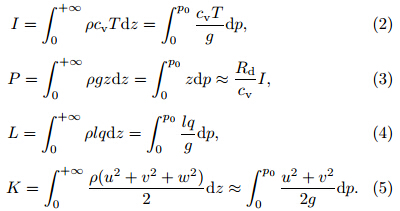
The vertically integrated thermal/dynamic features of the atmosphere can be extrapolated fromthe atmospheric energy. Following Peixoto and Oort(1992),the total atmospheric energy(EA)can be divided into four parts:
whereI,P,L, and K denote internal,potential,latent, and kinetic energy,respectively. Column integralmass weighted values are calculated as follows:Here,ρ is the density of air(kgm-3),cv is the atmospheric specific heat at constant volume(approximately 717 J kg−1 K−1),Rd is the gas constant fordry air(287 Jkg−1 K−1),l is latent heat of evaporation,Tis air temperature(K),zis the height of airmass above the earth surface(m),qis the mass ratioof water vapor(kg kg−1), and u,v, and ware zonal,meridional, and vertical wind speed,respectively(ms−1). The constant proportion between I and PinEq.(3)is accurate only if hydrostatic equilibrium isassumed, and the ratio should beRd/cv only if theeffect of water vapor has been neglected. Lis proportional to the precipitable water in the air column.Lalso depends on the particular phase transition; inmost situations,the main release of latent heat occursin rain, and l =le(2.6×10²Jkg−1)will be an appropriate value to use in Eq.(4). To connect the changeof atmospheric energy with the climate energy budget,the unit of the linear trend for atmospheric energy hasbeen written as W m-2(1 W m-2= 3.15×10⁹Jm−2per 100 yr)in this study.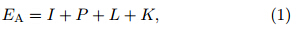
Kinetic energy will not be considered in thisstudy; consequently,only the thermal features ofatmospheric energy are presented. The magnitudeof kinetic energy is much smaller than the otherthree terms. Note that the kinetic energy in atmospheric transient eddies are comparable with thatin monthly mean circulations over the midlatitudinalzones(Chang et al., 2013). Therefore,a proper consideration of kinetic energy requires sub-daily simulationdata,which is not available for all models used in thisstudy.3. Spatial patterns of climatological mean atmospheric energy
In this section,the spatial patterns of climatological mean atmospheric energy will be discussed. FromEqs.(2)–(5),it is evident that atmospheric energyis controlled by both the corresponding atmosphericvariables(temperature,geopotential height, and specific humidity) and the atmospheric column depth.The local depth of the atmospheric column is primarily determined by the l and -surface geopotentialheight,which does not change significantly over time.Therefore,the distribution of climatological mean atmospheric energy from the models’ ensemble mean isquite close to that from reanalysis(Fig. 1). In particular,atmospheric energy is small over the regions withhigh altitude terrain,such as the Tibetan Plateau.The largest values for internal energy are given bythe models’ ensemble mean and NCEP/NCAR overnorthern Australia,northern Africa, and central SouthAmerica. Large potential and latent energy are foundover tropical regions; however,the latent energy seemsto be modified by the sea surface temperature.
 |
| Fig. 1. Climatological mean atmospheric energy patterns(1958–2000)derived from the ensemble mean of the models(first row) and two reanalysis datasets(second and third row). Contour intervals for the(a,d,g)internal energy,(b,e,h)potential energy, and (c,f,i)latent energy are 1×108,1×107, and 1×10⁷Jm-2,respectively. |
The intercomparison of spatial patterns of clima-tological mean atmospheric energy between singlemodel and reanalysis is shown as Taylor diagrams inFig. 2. Before constructing the Taylor diagrams,allmodels’ climatological mean atmospheric energy wasre-gridded to 2.5° ×2.5°. The spatial pattern correlation coefficient for all models and reanalysis data ishigher than 0.95. The spatial deviation of mean internal energy is also similar between the models and reanalysis, and it is more similar than that for SAT.In most models,the spatial deviation of the climatological mean potential energy is greater than that inERA-40 but smaller than in NCEP/NCAR. For latentenergy,the spatial deviation given by most models isgreater than that in NCEP/NCAR but smaller thanin ERA-40. Generally,the spatial patterns of simulated climatological mean atmospheric energy are wellreproduced by most models.
 |
| Fig. 2.Taylor diagrams for the climatological mean atmospheric(a)internal energy,(b)potential energy,(c)latentenergy, and (d)SAT. The correlation is represented by pattern correlation coefficients between models and reanalysis.The deviation means the difference between the local value and the global mean. The red and blue dots indicate theintercomparison results between models and NCEP/NCAR, and between models and ERA-40,respectively. |
The st and ardized series of globally averaged atmospheric energy are given in Figs. 3a–c. For themodels’ ensemble mean,all three atmospheric energyvalues decreased from 1958 to 1964 and then increasedcontinually except for two rapid declines in 1983 and 1992. The decrease of atmospheric energy in 1964,1983, and 1992 corresponded to the cooling aroundthe same time near the earth’s surface(Fig. 3d) and as likely caused by major volcanic eruptions in lowlatitudinal zones,i.e.,Agung(8°S),Fern and ina(0°S), and Mount Pinatubo(15°N),respectively(Robock,2000). Volcanic aerosols modulate atmospheric aerosoloptical depth and alter the energy budget of climatesystems(Sato et al., 1993). The simulated globally averaged internal energy is highly correlated withSAT. This suggests that the overall atmosphere temperature has increased because of barotropic effectson the global scale. Because the global atmosphereis generally in hydrostatic equilibrium and followsthe Clausius–Clapeyron equation,similar variation ofglobally averaged potential and latent energy is reasonable.
 |
| Fig. 3.Annual variations of globally averaged atmospheric(a)internal energy,(b)potential energy,(c)latent energy, and (d)SAT. All series have been st and ardized. Results from individual models are presented as thin-dashed lines withdifferent colors. Colors match those of the model names listed on the right. The results of the models’ ensemble mean(ESM,red) and two reanalysis datasets(ERA-40,blue; NCAP/NCAR,green)are given as thick solid lines. |
Regardless of the interannual variation,the internal and potential energy given by the two reanalysisdatasets have variations similar to the models’ ensemble mean,especially for the three cooling events. How-ever,there is a significant difference in latent energybetween productions of the two reanalyses. During thewhole period,the latent energy in ERA-40 is linearlyincreased. The NCEP/NCAR results show a sharp decrease from 1958 to 1964 with no linear increase after1971. In the following section,globally averaged atmospheric energy statistics from climate models and reanalysis data will be compared in further detail.4.1 Internal energy
Compared with reanalysis datasets,it seems thatmost models underestimate the climatological meaninternal energy. The climatological mean globally averaged I(Fig. 4a)is approximately 1.72×10⁹ Jm−2for most models,which is slightly smaller than thatfrom NCEP/NCAR(1.73×109 Jm−2) and ERA-40(1.74×10⁹ Jm−2). One exception is CSIRO-MK-360,which gives a climatological mean internal energy ofapproximately 1.78×10⁹ Jm−2.
Compared with climatological mean,the lineartrends of simulated internal energy are widely distributed among all models. The largest trend isgiven by the second realization of IPSL-CM5A-LR(4.7×10⁻³ Wm-2). The first realization of CSIRO-MK-360 and the second realization of HadGEM2-ESboth give a negative but insignificant trend. It shouldbe noted that the SAT trends for all realizations arepositive and significant(Fig. 4d). The weaker warming of the entire atmosphere rather than warming nearthe earth’s surface can be attributed to cooling in thestratosphere due to ozone reduction(figure omitted,refer to Santer et al., 1996). The trend of the models’ ensemble mean(1.9×10⁻³ Wm-2)isgreaterthanthat in ERA-40(1.7×10⁻³ Wm-2)but smaller thanin NCEP/NCAR(3.1×10-3 Wm-2).
 |
| Fig. 4.Climatological means(ordinate)versus linear trends(abscissa)of the globally averaged(a)internal energy,(b)potential energy,(c)latent energy, and (d)SAT for the period 1958–2000. The models’ ensemble mean is presented as ablue box. The horizontal width of the box indicates the root mean st and ard deviation among all models’ climatologicalmeans. The upper and lower boundary of the box shows where the lower 25% and upper 75% values are located for alllinear trends. The ensemble mean of linear trends among all models are indicated by the horizontal bar inside the box.The dashed error bar is the range of trends for all models. The results of ERA-40 and NCEP/NCAR are presented asblack open circle and diamond,respectively. |
Following the hydrostatic equilibrium assumptionfor atmosphere(Eq.(3)),the climatological meanglobally averaged potential energy should be proportional to internal energy. However,the climatologicalmeans of potential energy reproduced by climate models are separated into two groups. There are 20 modelsin the first group,all of which tend to give a lower climatological mean potential energy of approximately7.1×108 Jm−2; the remaining 12 models’ climatological mean potential energy is approximately 7.4×10⁸ Jm−2. The models’ ensemble mean result is about7.2×108 Jm−2,which is not close to any single model’sresult. The cause of the variation in the results of themodels cannot be ascertained in this study; however,ithas no relation with resolution of the models(neitherhorizontal nor vertical resolution). The results fromthe two reanalysis datasets are both approximately7.4×108 Jm−2,which is closer to result from the second group of models.
The trends of potential energy for most models are within the range of 0.5×10⁻³–1.0×10⁻³ Wm-2 . The trend from the models’ ensemble meanis 0.9×10⁻³ Wm-2 . This is acceptable because thetrend from ERA-40 and NCEP/NCAR is 0.7×10⁻³ and 1.4×10⁻³ Wm-2,respectively. The potentialenergy in the first realization of CSIRO-MK-360 decreases linearly,which means that the dry static atmospheric energy decreased between 1958 and 2000.Although with a decrease of internal energy,the potential energy from HadGEM2-ES(first realization)increases linearly. This is against the requirement ofthe hydrostatic equilibrium. 4.3 Latent energy
Latent energy is the potential energy that is released when water vapor in the atmosphere condenses.Latent energy is essential to climate change becausewater vapor is one of the most important naturalgreenhouse gas. The simulated climatological meanlatent energy ranges from 4.7×10⁷(IPSL-CM5A-LR)to 5.9×10⁷(CMCC-CESM)J m-2. The Inmcm4model is not included in the analysis because its specific humidity is obviously erroneous(e.g.,being negative)at somewhere. The models’ ensemble meanresult is 5.2×10⁷Jm−2,which is equal to that inNCEP/NCAR(5.2×107 Jm−2)but smaller than inERA-40(5.4×10⁷Jm−2).
Different from internal and potential energy,allmodels in this study show a linear increase of latent energy for the whole atmosphere,even for CSIRO-MK-360 and HadGEM2-ES. In other words,the CMIP5models are more likely to show an atmospheric moistening than global atmospheric warming or expansionduring historical climate change. ERA-40 gives atrend of approximately 3.2×10⁻³ Wm-2,whichisclose to the result obtained with FGOALS-s2. Thetrend from NCEP/NCAR is –0.6×10⁻³ Wm-2 . Sucha disagreement in the two reanalysis datasets has beenreported by Trenberth et al.(2005), and because theresult from ERA-40 is supported by that obtained withRSS SSM/I,the linear increase of latent energy seemsto be more reliable. Moreover,we also calculatedthe trend using the 20th century reanalysis datasets(Compo et al., 2011), and a statistically significant(>95% confidence level)positive trend of 0.89×10⁻³ Wm-2 for global latent energy is suggested. Therefore,it is reasonable to conclude that most models canproperly reproduce the moistening of the entire atmosphere for the period 1958–2000.
Although the climatological mean of latent energy is much smaller,its linear trends are comparableto those of internal and potential atmospheric energy.In other words,the increase ratio of latent energy ismuch greater than that of internal or potential energy.For the models’ ensemble mean,the latent energy ofthe atmosphere has increased by approximately 7.9%during 1958–2000; whereas the increase ratio of internal and potential energy is approximately 0.4%. Thisindicates that among internal,potential, and latentenergy,atmospheric latent energy is the most sensitiveto climate change,which may explain the importantrole that water vapor has played in climate feedbackstudies(Held and Soden, 2000,2006).4.4 Surface air temperature
SAT is widely used to indicate climate change;therefore,we also need to axamine this variable in atmospheric energy simulations. From Fig. 4d,it can beseen that the variation of simulated globally averagedSAT is quite close to the reanalysis results. The modelresults for climatological SAT mean range from 285.9(IPSL-CM5A-LR)to 288.5 K(GISS-E2-H). The models’ ensemble mean result is 286.9 K,which is quiteclose to that of NCEP/NCAR(287 K) and smallerthan that of ERA-40(287.5 K). Note that the descriptions of SAT in the two reanalysis products are identical except for the Arctic and Antarctic regions(figureomitted)(Jones et al., 1999; Simmons et al., 2004).
Because all climate models’ globally averagedSAT shows a positive trend during 1958–2000,airwarming near the earth surface appears to be a moreconfident result than warming of the whole atmosphere. The weakest warming appears in the fifth realization of CSIRO-MK-360(0.37 K per 100 yr),whilethe strongest warming appears in FGOALS-s2(2.4 Kper 100 yr). The trend of the models’ ensemble meanis 1.38 K per 100 yr,which is larger than that of ERA-40(1.1 K per 100 yr) and NCEP/NCAR(0.9 K per100 yr). Therefore,most models seem to overestimatethe increase of SAT during 1958–2000.
For the globally averaged climatological mean atmospheric energy,the results of the models’ ensemble mean are closer to that from NCEP/NCAR. Withregard to the linear trend for the period 1958–2000,the result from the models’ ensemble mean seems tobe closer to that from ERA-40. These features canalso be found in SAT. Note that the identification ofglobally averaged SAT between the models’ ensemblemean and reanalysis is more significant than that foratmospheric energy. Thus,climate change near theearth’s surface in the past decades seems to be betterunderstood, and therefore can be well reproduced bynumerical models. With regard to the thermal stateof the entire climate subsystems(e.g.,atmospheric energy),considerable uncertainty remains. 5. Globally averaged atmospheric energy connections
On the basis of the above discussion,the globallyaveraged atmospheric energy and SAT show greaterdifferences than other features in most models. Therefore,before proceeding with the discussion presentedin this section,the simulated atmospheric energyneeds to be normalized first. Because the globallyaveraged SAT is often used to represent the thermalstate of climate,all atmospheric energy statistical results are normalized with the statistics of SAT.
The climatological mean of internal and potential energy does not demonstrate any connections evenafter being normalized. The two groups of modelswith different potential energy values are still significant,as shown in Fig. 5a. However,the normalized mean latent energy shows a linear correlation(atthe 95% confidence level for t-test)with internal energy among all models(Fig. 5b); the ratio is approximately 3.6×10⁻². Considering that the difference inthe climatological mean globally averaged SAT is smallamong all models,this linear relationship means thatif the climatological mean internal energy in a model islarger than the models’ ensemble mean for 100 J m-2,its mean latent energy should be approximately 3.6 Jm−-2greater. This relationship is also supported bythe two reanalyses. Therefore,assuming equal globalmean SAT,when the atmosphere has greater internalenergy,its latent energy rather than potential energywill also be greater.
| |
| Fig. 5.Distributions of(a,b)climatological mean,(c,d)linear trend, and (e,f)root mean st and ard deviation(RMSD)between different models(a,c,e: globally averaged internal vs. potential energy; b,d,f: globally averaged internalvs. latent energy). Results for individual models are denoted as black dots. Results from ERA-40 and NCEP/NCARare denoted as open box and circle,respectively. All atmospheric energy statistics have been normalized with thecorresponding SAT statistics(i.e.,units for all axes are 106JK-1 m-2). The linear fitted line for all models is alsogiven. The slopes of fitted line in(a)–(f)are –4.8×10-2,3.6×10-2,0.30,0.31,0.30, and 0.31,respectively. |
The linear connections between normalized atmospheric energy trends are statistically significant(at>99% confidence level). From Fig. 5c,it can be seenthat the ratio between normalized potential energy and internal energy is 0.30. This means that underthe same warming rate near the earth’s surface,theincrease of atmospheric potential energy is approximately 30% of that of internal energy. This result iswell supported by the two reanalysis datasets. Considering that the ratio of climatological mean of potentialenergy to that of internal energy is approximately 0.4(Eq.(3)),the ratio of the normalized trend betweeninternal and potential energy implies that the atmosphere will be more compressed and the hydrostaticalequilibrium is destroyed in the models’ representationof historical climate change.
The ratio of the trend between simulated latent and internal energy,derived from all models exceptInmcm4,is approximately 0.31(Fig. 5d). This result is statistically significant at the 99% confidencelevel. Because the climatological mean of latent energy is two orders of magnitude smaller than that ofinternal energy,such a result indicates that under acertain increase of global SAT,the increase of latentenergy is most intensive. However,the two reanalyses do not appear to agree with the models. Theresult from ERA-40 indicates an even greater increaseof latent energy and the result from NCEP/NCAR indicates that the atmosphere has become hot and dryduring past decades.
The root mean st and ard deviation(RMSD)of theatmospheric energy time series is similar to those of thetrend(Figs. 5e and 5f). The ratio of RMSD betweenpotential and internal energy as well as that betweenlatent and internal energy from models are close tothat of the trend. Therefore,the change of differentglobal atmospheric energy will maintain a constant ratio on both short(interannual) and longer(decadal)timescales in CMIP5. Note that the RMSD of latentenergy from NCEP/NCAR is still much weaker thanthat of the potential energy. 6. Conclusions and discussion
In this study,we investigated atmospheric energyin historical climate change(1958–2000)to evaluate32 CMIP5 climate models. The main conclusions aresummarized below:
(1)The spatial patterns of climatological meanatmospheric energy reproduced by most models arequite similar to those of the two reanalysis datasets(ERA-40 and NCEP/NCAR).
(2)The globally averaged internal and potentialenergy from the models’ ensemble mean have similar variations to those of ERA-40 and NCEP/NCARduring 1958–2000, and the globally averaged latentenergy from the models’ ensemble mean is close tothat of ERA-40.
(3)The climatological mean of globally averagedatmospheric energy from the models’ ensemble meanis close to that from NCEP/NCAR,while the trendsfrom the CMIP5 model simulations are close to thatfrom ERA-40.
(4)Under equal warming conditions near theearth’s surface,the ratio of trends between simulatedpotential and internal energy is 0.30. The comparableratio of trends between latent and internal energy is0.31. Considering the comparison of climatologicalmean values of atmospheric energy,these two ratiosindicate that the proportion of latent energy in theentire atmospheric energy has increased while that ofpotential energy has decreased under historical globalwarming.
The significant spread of atmospheric energy inclimate models and two reanalysis datasets should benoted. The simulation ability of climate models hasimproved during the past two decades,which seems tobe supported by the more realistic change of SAT inCMIP5 models(Fig. 4d). However,for atmosphericenergy,the results from two reanalyses diverge significantly. A significant cause of the uncertainty inatmospheric energy may be that the physical constraint of conservation of dry air mass is violated in thetwo reanalyses with increasing magnitude prior to theassimilation of satellite data(Trenberth and Smith, 2005). Similarly,a determination of atmospheric massis also needed to underst and the distribution of atmospheric energy among all climate models.Acknowledgments.
We acknowledge theWorld Climate Research Programme’s climate modeling groups for producing and making their modeloutputs available. We also appreciate all comments and help from the reviewers and editors. The authorswould like to thank Enago(www.enago.cn)for theEnglish language review.
| [1] | Alessandri, A., P. G. Fogli, M. Vichi, et al., 2012: Strengthening of the hydrological cycle in future scenarios: Atmospheric energy and water balance perspective. Earth System Dynamics, 3, 199-212, doi: 10.5194/esd-3-199-2012. |
| [2] | Allen, M. R., P. A. Stott, J. F. B. Mitchell, et al., 2000: Quantifying the uncertainty in forecasts of anthro-pogenic climate change. Nature, 407, 617-620, doi:10.1038/35036559. |
| [3] | Allen, M. R., and P. A. Stott, 2003: Estimating signal am-plitudes in optimal fingerprinting. Part I: Theory. Climate Dyn., 21, 477-491, doi: 10.1007/s00382-003-0313-9. |
| [4] | Annamalai, H., K. Hamilton, and K. R. Sperber, 2007: The South Asian summer monsoon and its relation-ship with ENSO in the IPCC AR4 simulations. J. Climate, 20, 1071-1092, doi: 10.1175/Jcli4035.1. |
| [5] | Baettig, M. B., M. Wild, and D. M. Imboden, 2007: A climate change index: Where climate change may be most prominent in the 21st century. Geophys. Res. Lett., 34, doi: 10.1029/2006GL028159. |
| [6] | Baldwin, M. P., M. Dameris, and T. G. Shepherd, 2007: Atmosphere——How will the stratosphere af-fect climate change? Science, 316, 1576-1577, doi:10. 1126/science.1144303. |
| [7] | Barnett, T. P., K. Hasselmann, M. Chelliah, et al., 1999: Detection and attribution of recent climate change: A status report. Bull. Amer. Meteor. Soc.,80, 2631-2659, doi: 10.1175/1520-0477(1999)080. |
| [8] | Barnett, T. P., D. W. Pierce, and R. Schnur, 2001: Detec-tion of anthropogenic climate change in the world's oceans. Science, 292, 270-274, doi: 10.1126/sci-ence.1058304. |
| [9] | Bodri, L., and V. Cermak, 2005: Borehole temperatures, climate change and the pre-observational surface air temperature mean: Allowance for hydraulic condi-tions. Global Planet. Change, 45, 265-276, doi:10.1016/j.gloplacha.2004.09.001. |
| [10] | Bony, S., R. Colman, V. M. Kattsov, et al., 2006: How well do we understand and evaluate climate change feedback processes? J. Climate, 19, 3445-3482, doi:10.1175/Jcli3819.1. |
| [11] | Chamberlin, T. C., 1897: A group of hypothesis hear-ing on climatic change. J. Geol., 5, 653-683, doi:10.1086/607921. |
| [12] | Chang, E. K. M., Y. J. Guo, X. M. Xia, et al., 2013: Storm-track activity in IPCC AR4/CMIP3 model simulations. J. Climate, 26, 246-260, doi:10.1175/Jcli-D-11-00707.1. |
| [13] | Church, J. A., and N. J. White, 2006: A 20th century acceleration in global sea-level rise. Geophys. Res. Lett., 33, doi: 10.1029/2005gl024826. |
| [14] | Compo, G. P., J. S. Whitaker, P. D. Sardeshmukh, et al., 2011: The twentieth century reanalysis project. Quart. J. Roy. Meteor. Soc., 137, 1-28, doi: 10.1002/Qj.776. |
| [15] | Dixon, K. W., and J. R. Lanzante, 1999: Global mean surface air temperature and North Atlantic over-turning in a suite of coupled GCM climate change experiments. Geophys. Res. Lett., 26, 1885-1888, doi: 10.1029/1999gl900382. |
| [16] | Fleming, J. R., 2005: Historical Perspectives on Climate Change. Oxford University Press, 208 pp. |
| [17] | Hansen, J., L. Nazarenko, R. Ruedy, et al., 2005: Earth's energy imbalance: Confirmation and impli-cations. Science, 308, 1431-1435, doi: 10.1126/sci-ence.1110252. |
| [18] | Held, I. M., and B. J. Soden, 2000: Water vapor feedback and global warming. Annu. Rev. Energ. Env., 25,441-475, doi: 10.1146/annurev.energy.25.1.441. |
| [19] | Held, I. M., and B. J. Soden, 2006: Robust responses of the hydrological cycle to global warming. J. Climate, 19, 5686-5699, doi: 10.1175/Jcli3990.1. |
| [20] | Henderson-Sellers, A., R. E. Dickinson, T. B. Durbidge, et al., 1993: Tropical deforestation-modeling local-scale to regional-scale climate change. J. Geophys. Res., 98, 7289-7315, doi: 10.1029/92jd 02830. |
| [21] | Ingram, W. J., C. A. Wilson, and J. F. B. Mitchell, 1989: Modeling climate change——An assessment of sea ice and surface albedo feedbacks. J. Geophys. Res., 94,8609-8622, doi: 10.1029/Jd 094id06p08609. |
| [22] | Johannessen, O. M., L. Bengtsson, M. W. Miles, et al., 2004: Arctic climate change: Observed and mod-elled temperature and sea-ice variability. Tellus A,56, 328-341, doi: 10.1111/j.1600-0870.2004.00060.x. |
| [23] | Jones, P. D., M. New, D. E. Parker, et al., 1999: Sur-face air temperature and its changes over the past 150 years. Rev. Geophys., 37, 173-199, doi: 10.1029/1999rg900002. |
| [24] | Kalnay, E., M. Kanamitsu, R. Kistler, et al., 1996: The NCEP/NCAR 40-year reanalysis project. Bull. Amer. Meteor. Soc., 77, 437-471, doi: 10.1175/1520-0477(1996)077. |
| [25] | Kiehl, J. T., and K. E. Trenberth, 1997: Earth's annual global mean energy budget. Bull. Amer. Me-teor. Soc., 78, 197-208, doi: 10.1175/1520-0477 (1997)078. |
| [26] | Levitus, S., 2000: Warming of the world ocean. Sci-ence, 287, 2225-2229, doi: 10.1126/science.287.5461.2225. |
| [27] | Levitus, S., J. Antonov, and T. Boyer, 2005: Warming of the world ocean, 1955-2003. Geophys. Res. Lett.,32, doi: 10.1029/2004gl021592. |
| [28] | Li, Z. Q., and H. G. Leighton, 1993: Global climatologies of solar-radiation budgets at the surface and in the atmosphere from 5 years of ERBE data. J. Geophys. Res., 98, 4919-4930, doi: 10.1029/93jd00003. |
| [29] | Lucarini, V., and F. Ragone, 2011: Energetics of cli-mate models: Net energy balance and meridional enthalpy transport. Rev. Geophys., 49, doi: 10.1029/2009rg000323. |
| [30] | Mayer, M., and L. Haimberger, 2012: Poleward atmo-spheric energy transports and their variability as evaluated from ECMWF reanalysis data. J. Cli-mate, 25, 734-752, doi: 10.1175/Jcli-D-11-00202.1. |
| [31] | Meehl, G. A., W. M. Washington, W. D. Collins, et al., 2005: How much more global warming and sea level rise? Science, 307, 1769-1772, doi: 10. 1126/sci-ence.1106663. |
| [32] | Meehl, G. A., C. Covey, K. E. Taylor, et al., 2007: THE WCRP CMIP3 multimodel dataset: A new era in climate change research. Bull. Amer. Meteor. Soc.,88, 1383-1394, doi: 10.1175/bams-88-9-1383. |
| [33] | Nobre, C. A., P. J. Sellers, and J. Shukla, 1991: Amazonian deforestation and regional climate change. J. Climate, 4, 957-988, doi: 10.1175/1520-0442(1991)004<0957:Adarcc>2.0.Co;2. |
| [34] | Oreskes, N., 2004: Beyond the ivory tower——The scien-tific consensus on climate change. Science, 306,1686, doi: 10.1126/science.1103618. |
| [35] | Peixoto, J. P., and A. H. Oort, 1992: Physics of Climate. American Institute of Physics, 520 pp. |
| [36] | Robock, A., 2000: Volcanic eruptions and climate. Rev.Geophys., 38, 191-219, doi: 10.1029/1998rg000054. |
| [37] | Santer, B. D., K. E. Taylor, T. M. L. Wigley, et al., 1996: A search for human influences on the thermal structure of the atmosphere. Nature, 382, 39-46, doi: 10.1038/382039a0. |
| [38] | Santer, B. D., T. M. L. Wigley, C. Mears, et al., 2005: Amplification of surface temperature trends and variability in the tropical atmosphere. Science, 309,1551-1556, doi: 10.1126/science.1114867. |
| [39] | Sato, M., J. Hansen, P. Mccormick, et al., 1993: Strato-spheric aerosol optical depths, 1850-1990. J. Geophys. Res., 98, 22987-22994, doi: 10.1029/93jd02553. |
| [40] | Simmons, A. J., P. D. Jones, V. da Costa Bechtold, et al., 2004: Comparison of trends and low-frequency variability in CRU, ERA-40, and NCEP/NCAR analyses of surface air temperature. J. Geophys. Res., 109, doi: 10.1029/2004jd005306. |
| [41] | Soden, B. J., and I. M. Held, 2006: An assess-ment of climate feedbacks in coupled ocean-atmosphere models. J. Climate, 19, 3354-3360, doi: 10.1175/Jcli3799.1. |
| [42] | Stott, P. A., G. S. Jones, and J. F. B. Mitchell, 2003: Do models underestimate the solar contri-bution to recent climate change? J. Climate, 16,4079-4093, doi: 10.1175/1520-0442(2003)016. |
| [43] | Taylor, K. E., R. J. Stouffer, and G. A. Meehl, 2012: An overview of CMIP5 and the experiment de-sign. Bull. Amer. Meteor. Soc., 93, 485-498, doi:10.1175/Bams-D-11-00094.1. |
| [44] | Trenberth, K. E., and L. Smith, 2005: The mass of the atmosphere: A constraint on global analyses. J. Climate, 18, 864-875, doi: 10.1175/Jcli-3299.1. |
| [45] | Trenberth, K. E., J. T. Fasullo, and L. Smith, 2005: Trends and variability in column-integrated atmo-spheric water vapor. Climate Dyn., 24, 741-758, doi: 10.1007/s00382-005-0017-4. |
| [46] | Trenberth, K. E., J. T. Fasullo, and J. T. Kiehl, 2009: Earth's global energy budget. Bull. Amer. Meteor. Soc., 90, 311-323, doi: 10.1175/2008bams2634.1. |
| [47] | Uppala, S. M., P. W. KAllberg, A. J. Simmons, et al., 2005: The ERA-40 reanalysis. Quart. J. Roy. Me-teor. Soc., 131, 2961-3012, doi: 10.1256/Qj.04.176. |
| [48] | Watterson, I. G., M. R. Dix, and R. A. Colman, 1999: A comparison of present and doubled CO2 climates and feedbacks simulated by three general circulation models. J. Geophys. Res., 104, 1943-1956, doi:10.1029/1998jd200049. |
| [49] | Wielicki, B. A., B. R. Barkstrom, E. F. Harrison, et al., 1996: Clouds and the earth's radiant energy system (CERES): An earth observing system experiment. Bull. Amer. Meteor. Soc., 77, 853-868. |
| [50] | Willmott, C. J., and D. R. Legates, 1993: A compar-ison of GCM-simulated and observed mean Jan-uary and July surface air temperature. J. Cli-mate, 6, 274-291, doi: 10.1175/1520-0442(1993)006. |
| [51] | Zhang, X., F. W. Zwiers, G. C. Hegerl, et al., 2007: Detection of human influence on twentieth-century precipitation trends. Nature, 448, 461-465, doi:10.1038/nature06025. |
| [52] | Zhou, T. J., and R. C. Yu, 2006: Twentieth-century surface air temperature over China and the globe simulated by coupled climate models. J. Climate,19, 5843-5858, doi: 10.1175/Jcli3952.1. |