 2014, Vol. 28
The Chinese Meteorological Society
Article Information
- LIU Yan, XUE Jishan. 2014.
- Assimilation of Global Navigation Satellite Radio Occultation Observations in GRAPES: Operational Implementation
- J. Meteor. Res., 28(6): 1061-1074
- http://dx.doi.org/10.1007/s13351-014-4027-1
Article History
- Received April 24, 2014;
- in final form June 17, 2014


2 State Key Laboratory of Severe Weather, Chinese Academy of Meteorological Sciences, China MeteorologyAdministration, Beijing 100081
Radio occultation(RO)is a limb-soundingremote-sensing technique used for measuring the physical properties of a planetary atmosphere. When aradio signal travels from a global navigation satellitesystem(GNSS)transmitter to a receiver in the low-earth orbit satellite, it is refracted. The delay or thechange of bending due to the atmospheric refractioncan be precisely measured, and then used to infer theelectron density in the ionosphere and the refractivitycontaining temperature and water vapor informationin the stratosphere and troposphere. Compared withother satellite remote-sensing observations, RO observations have the advantage of high accuracy, high vertical resolution, all-weather global coverage, no systembias, etc. They therefore have great potential value inweather and climate applications(Eyre, 1994; Ware et al., 1996; Kursinski et al., 1997; Anthes et al., 2000;Wickert et al., 2001).
Many advanced numerical weather prediction(NWP)centers, such as the European Centre forMedium-Range Weather Forecasts, have shown thatoccultation data are one of the most important setsof observations in the global observation system, asthey can significantly improve the analysis and forecast quality for both the Northern and Southern Hemispheres, particularly the Southern Hemisphere and the stratosphere where conventional observations arescarce(e. g., Healy et al., 2005; Cucurull et al., 2006;Aparicio and Deblonde, 2008; Buontempo et al., 2008;Cucurull and Derber, 2008; Healy, 2008; Poli et al., 2009; Rennie, 2010). In addition, RO observations donot require bias correction; they can "anchor" the biascorrection applied to satellite radiances and help identify NWP model biases(Collard and Healy, 2003).
Although early occultation experiments(Healy and Thepaut, 2006)proved RO observations' potentialcontribution to NWP, it was not until the launch ofFORMOSAT-3/COSMIC(Formosa Satellite mission3/Constellation Observation System for Meteorology, Ionosphere, and Climate; simply referred to as COS-MIC hereafter)in April 2006 that the operational assimilation of RO data became a reality. The mainreason is that the COSMIC mission consists of six loworbit satellites, which can provide more RO observations(approximately 2000 profiles daily), and the dataare available in near real time, with less than 3 h of latency(Anthes et al., 2008). Besides, two operationalRO missions, i. e., the METOP-A launched in October 2006(Loiselet et al., 2000) and the METOP-Blaunched in September 2012, provide more than 1300profiles daily. Other research RO missions, such asCNOFS and TerraSAR-X(Wickert et al., 2005, 2008), also provide a considerable number of RO observations.
GRAPES(Global/Regional Assimilation and PrEdiction System)is the new generation operationalNWP system of the China Meteorological Administration(CMA). It was developed in response to anincreasingly urgent need for more accurate numerical weather forecasts in recent years(Xue, 2006; Xue and Chen, 2008). The regional and global GRAPESsystems have been run in routine operation or pre-operation in the National Meteorological Center ofCMA. As a new type of satellite observation, the ROdata and their assimilation into the GRAPES are discussed in detail in this paper, including the design ofthe observation operator, the strategy of operationalimplementation, and analysis of the assimilation impact on forecast experiments.
The remainder of this paper is organized as follows. Section 2 provides a simple description of theGRAPES variational assimilation system(GRAPES-Var). Section 3 describes the RO observation preprocessing system. Section 4 elaborates on the RO refractivity observation operator and observation error. Sections 5 and 6 present the results of short- and long-term RO observation assimilation experiments, respectively. A summary of the key findings and further discussion are presented in the final section. 2. GRAPES-Var
The early GRAPES-Var(Zhuang et al., 2005; Xue et al., 2008)did not match the GRAPES forecastmodel in either the type of coordinate used or the analyzed atmospheric state vectors. This caused manyerrors in coordinate and variable transformations. Recently, we have updated the GRAPES-Var from thepressure coordinate to the terrain-following height coordinate(Xue et al., 2012). Namely, the current definition of the coordinate and atmospheric state variables in GRAPES-Var is completely consistent withthe GRAPES forecast model; the initial field is obtained directly after data assimilation and without anyadditional transformation. Therefore, the state vectors are
where u and v are the components of wind, q is specific humidity, and m denotes the mass field, whichis either Exner pressure π or potential temperatureθ. Although GRAPES is a non-hydrostatic model, we do not consider the non-hydrostatic problem ofGRAPES-Var at present, and we choose π as the statevariable and θ as the derivative of π. We also do notanalyze hydrometeors. Figure 1 presents a schematicdiagram of the atmospheric state and analysis variables of new GRAPES-Var in the Charney-Phillipsvertical grid. The expression of the RO observationoperator is required to suit such a definition of thecoordinate and variables.
 |
| Fig. 1. Schematic diagram of the atmospheric state and analysis variables of GRAPES-Var in the Charney-Phillipsvertical grid. [From Xue et al., 2012] |
The RO measurements under different data processing stages, from the phase and amplitude, bendingangle, and refractivity, to the retrieval of the temperature and water vapor pressure, can be assimilated. The favorite RO measurements assimilated in an operational NWP system are ionosphere-corrected bending angles and refractivity(Eyre, 1994; Kuo et al., 2000). The calculation of bending angle is affected bythe height of the model top(Aparicio and Deblonde, 2008; Rennie, 2010); therefore, refractivity is the bestchoice for current GRAPES with the relatively lowmodel top of 32. 5 km. 3. 1 Conversion of the coordinate
WGS84(World Geodetic System 1984)is a coordinate system designed for GNSS satellites. Occultation observations are reported based on the WGS84geoid geometric altitude, whereas GRAPES employsthe geopotential height vertical coordinate. Therefore, we first need to convert the geometric altitudeto geopotential height for RO observations in the datapreprocessing. The conversion relation follows that of Rennie(2010). 3. 2 Quality control and data thinning
Before data assimilation, it is essential to applyquality control(QC)procedures. The most basic QCprocess is to reject the outliers that are away from themean status of most data. Three QC procedures areapplied in GRAPES. The dual weights mean and st and ard deviation method proposed by Lanzante(1996)is applied first for spatial consistency checks. This removes the refractivity observations that deviate fromthe bi-weight mean by more than five times the biweight st and ard deviation. It is performed over high(60°-90°N/S), medium(30°-60°N/S), and low(30°S-30°N)latitudinal belts for each vertical level. Thesecond QC procedure is to reject the data that couldpossibly contain super-refractions. Suspicious observations are below regions wheredN/dz< -50 N-unitkm-1 and d2N/d2z> 100(N-unit)2 km-2 are sequentially flagged. Here, N is refractivity and z is height(Poli et al., 2009).
The background check is not performed in the pre-processing but in the data assimilation system. Thecriterion used in the background field check is
where the subscripts o and b represent the observation and background, and σo is the observation error st and ard deviation.
Since the vertical resolution of the occultationdata is much higher than that of the model, theymust be thinned. Our approach is to assimilate oneobservation nearest each vertical analysis level, whichnot only avoids the high correlation of observation errors, but also retains enough fine observation information.
In summary, the preprocessing procedure of ROdata is as follows. First, the data are read; then, the coordinates are converted from geometric altitudeto geopotential height, and quality control is per-formed; finally, the data are thinned in the verticaldirection. 4. Observation operator and observation error4. 1 Design of the observation operator
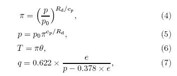
The observation operator of refractivity is expressed as
where N is the refractivity in N-unit, p is the pressurein hPa, T is the temperature in Kelvin, and e is thewater vapor pressure in hPa. Pressure, temperature, and water vapor pressure are not the atmospheric statevariables in GRAPES; instead, we use Exner pressure, specific humidity, and the wind components of u and v. Therefore, the calculation of Eq. (3)uses the formulaewhere cp = 1004. 5 J kg-1 K-1 is the specific heat capacity of dry air at constant pressure, Rd = 287. 05J kg-1 K-1 is the specific gas constant for dry air, and p0 = 1000 hPa is the reference surface pressure. Corresponding tangent linear operators areFinally, the tangent linear operator of refractivity isexpressed as


As a result of using the Charney-Phillips staggering grid, the pressure, temperature, and specific humidity are not on the same vertical level, the calculation of model refractivity is defined at the θ level. Thismeans that the error induced by the variable transformation and vertical interpolation is less, because weonly interpolate π; otherwise, we need to interpolateθ and q. The parameter π at the θ level is calculatedby assuming a linear variation of π with geopotentialheight:
Corresponding pressure at the θ level is then obtainedbased on Eq. (5).
The mean virtual temperature Tv at the θ level iscalculated by using the hydrostatic equation
where g = 9. 80665 m s-2 is the mean gravitationalacceleration.
As GRAPES uses the terrain-following height-based coordinate, the slope of the model level mightlead to a large horizontal interpolation error. Therefore, we first calculate the background refractivity profile of the four grid points nearest the lowest tangential point of occultation observation, and then use bilinear interpolation to obtain the background refractivity profile at this tangential point. Finally, we linearly interpolate lnN to the occultation observationlocation:
where
 , and the subscript at-obsdenotes the observation location. We do not take thedrift of the tangential point into account. 4. 2 Test of the observation operator
To test the correctness of the refractivity observation operator, we design an idealized experiment inwhich the observation is at the analysis grid point. The variational assimilation problem is attributed tosolving the following cost function:
where vector x represents the atmospheric state, xbis the background field, vector y represents the observations, B and O are the covariance matrices of thebackground and observations, H(x) represents the observation operator, and the superscript T represents amatrix transpose.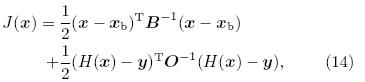
For a single observation, the analysis increment is
where H' is the tangent linear operator. Assumingthat the observation is a logarithm of refractivity and the analysis variable is π, Eq. (15)is expressed asWhen there is only one observation, the product ofthe vectors in the two brackets of the right-h and termis a definite value, and the profile of dπa depends onBπHT =(HBπ)T.

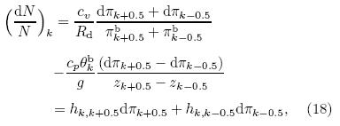
If the impact of moisture is ignored, that is, onlythe first part of Eq. (3)is considered, the tangentlinear operator is
Note the staggering relationship between N and π;thus, Eq. (17)should be expressed on the θ level:where hk, k+0+5 and hk, k-0+5 are the pressure coe±-cients at levels k+0. 5 and k-0. 5(observations are located at level k)Here, in Eqs. (19) and (20), the first subscript represents the location of the observation, and cv = cp-Rdis the specific heat capacity of dry air at constant volume. The pressure coe±cients at other levels are zeroexcept for these two levels.
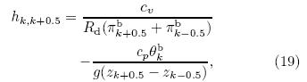
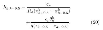
Based on the above equation, we test the correctness of the observation operator in GRAPES-1DVar, which has a consistent configuration with GRAPES-3DVar. Given the following parameters: No = 82. 339N-unit at level k = 21(equivalent to 10357 m), σo =0. 415 N-unit, θk = 333. 9 K, πk+0. 5 = 0. 649031, πk-0. 5= 0. 6732736, σπ = 0. 0004, zk+0. 5 = 10780 m, and zk-0. 5 = 9951 m, the numerical solution and modelsolution are found consistent(see Table 1).

The observation error of occultation refractivity isobtained according to the statistical result of Rennie(2010), which is a function of latitude and altitude. It is divided into three areas: low latitude(30°S-30°N), midlatitude(30°-60°N/S), and high latitude(60°-90°N/S). Figure 2 shows the st and ard deviation(σo)of normalized observation error of refractivity. Itis obtained by using the equation
where σ is the st and ard deviation of the normalizedobservation error, and is a function of latitude and height.
 |
| Fig. 2. Vertical profile of the st and ard deviation of normalized observation error for RO refractivity as a functionof height and latitude. The dotted line is for low latitudes(30°S-30±N), solid line for midlatitudes(30°-60°N/S), and dashed line for high latitudes(60°-90°N/S). The profile isadjusted based on the results of Rennie(2010). |
Two experiments with and without RO data assimilation are performed in the global GRAPES system. They are called the control experiment and theRO experiment. In the control experiment, only theconventional observations are assimilated, which include radiosonde, synop, ships, aircraft, and clouddrift wind observations. The RO experiment thenadds the COSMIC and METOP-A RO observationsto the basic observations of the control experiment. The horizontal resolution of the outer loop is 1°, and that of the inner loop is 1. 125°, correspondingto the spherical filter's cutoff wavenumber of T106. The length of the assimilation time window is 6 h. The incremental digital filter is used for the initialization. We employed the GRAPES forecast modelversion available by the end of 2011. The modeltop is 32. 5 km with 36 layers. The horizontal resolution is 1±. The time integration step is 600 s. The physical parameterizations include the WSM6(WRF Single-Moment 6-class)microphysics parameterization(Hong and Lim, 2006), RRTM(Rapid Radiative Transfer Model)radiation parameterization(Mlawer et al., 1997), CoLM(Common L and Model)l and surface parameterization(Dai et al., 2003), MRF(Medium-Range Forecast)planetary boundary layerparameterization(Troen and Mahrt, 1986), SAS(Simplified Arakawa-Schubert)mass flux parameterizationscheme(Arakawa and Schubert, 1974), and so on. Theexperiments run from 0000 UTC 1 July 2011 to 1800UTC 31 July 2011.
Figure 3a shows an example of the horizontaldistribution of RO profile locations. There are 404COSMIC occultation profiles(dots) and 118 GRAS(Global navigation satellite system Receiver for Atmospheric Sounding)occultation profiles(triangle)fromMETOP-A satellite within each assimilation window. The occultation events mainly occur in the mid-highlatitude areas because the COSMIC and METOP-Asatellites have a high inclination. Figure 3b shows thenumber of occultation data before and after the background quality check in each assimilation time windowin the RO experiment, and also the number of RO profiles(each profile contains several data). The averagenumber of RO profiles is about 464, with 14379 ROdata at each assimilation time window, and the average number of RO data is 12828 after the backgroundcheck. About 10. 8% of the RO data are rejected.
 |
| Fig. 3. (a)Coverage of RO data assimilated at 1200 UTC 4 July 2011. (b)Time evolution of RO data amount at theassimilation time window in the RO experiment from 0000 UTC 1 July to 1800 UTC 31 July 2011. The x-axis representstime, with 1 denoting 0000 UTC 1 July 2011 and 121 denoting 0600 UTC 31 July 2011. The y-axis on the left(right)represents the number of RO data(profiles). The solid black line represents the number of occultation profiles and thelines with circles and triangles represent the number of occultation data before and after quality control. |
In the one-month RO assimilation experiment, the percentage of RO observations is only about 9%, which is quite low, compared with 47% of atmosphericmotion vectors, 24% of radiosonde data, 16% of aircraft observations, etc., because the number of ROdata available in the global observing system is relatively small at present. However, the 9% occultation data surprised us in subsequent experiments, asit plays a very important role. 5. 2 Comparison with the observations
The impact of RO data on the analysis can beidentified by comparing the departure of the background and analysis to the observation(called BMO and AMO, respectively). Figure 4 shows the statistical results of the AMO and BMO profiles. Since themagnitude of refractivity from the surface to 30 km isabout 2, all the statistical computations are normalized by the observation error st and ard deviation. Thespecified observation error is reasonable, because theAMO profile is closer to zero than the BMO profile is, and the root-mean-square error(RMSE)of analysisis significantly reduced, indicating that the assimilation of occultation data has clearly a positive effect. The difference between BMO and AMO in the uppertroposphere and the stratosphere is larger, indicatingthat the model error is larger there. However, it canbe effectively controlled after the RO data are assim-ilated. The strongest effect is between 10 and 25 km, where the RO data have the highest accuracy; whilethe weaker effect is above 25 km and below 10 km. Besides the data accuracy; the error might be relatedto the vertical structure of GRAPES, especially nearthe model top.
 |
| Fig. 4. Mean bias(dashed line) and root-mean-squareerror(solid line)between the background/analysis fieldsof the RO experiment and the observation as a functionof geopotential height, which is normalized by observationerror st and ard deviation. The grey lines represent back-ground minus observation(BMO) and the black lines rep-resent analysis minus observation(AMO). |
The NCEP analysis data are used to evaluatethe impact of RO observation assimilation. GRAPESis a developing NWP system, in which the observation types assimilated are still limited; whereas theNCEP analysis data accommodate assimilation of avariety of satellite-remote sensing data, making it avaluable dataset to compare and examine the problems in GRAPES. Figure 5 presents comparisons between GRAPES and NCEP analysis. The geopotentialheight difference between the control experiment and the NCEP analysis is mainly located in the SouthernHemisphere, the stratosphere of the tropics, and thehigh latitudes in the Northern Hemisphere. These differences are clearly reduced after the RO observationsare assimilated. The difference between the RO experiment and the control experiment is similar to thatbetween the control experiment and the NCEP analysis, especially over 40°-70°S, where the number ofradiosonde and aircraft observations is only 5% of thedata in the same latitude zone in the Northern Hemisphere. As a result, once the RO observations areassimilated, a significant improvement in the analysis can be seen. The situation with respect to temperature analysis is similar to that of geopotentialheight. However, the gradient difference above 20 hPais larger, which might be related to the vertical structure of GRAPES, but this needs a further investigation.
For the wind analysis, the differences with and without the assimilated RO data are concentrated inthe tropics as well as in the Southern Hemisphere(Fig. 5d). The improvement in the wind analysis with ROobservation assimilation in the equatorial tropics isnot so obvious as that in the Southern Hemisphere(Fig. 5e). This illustrates that the wind analysis ofGRAPES in the tropical region is not good. Giventhe fact that the coupling between wind and pressurefields is weak in the tropics, and the RO data are inessence a type of thermal temperature observation, itis acceptable that the addition of RO observations exerted less of an impact on the wind analysis, and theimpact might have been offset by some systematic error if there is any.
 |
| Fig. 5. Comparisons between the control and the RO experiment for(a-c)geopotential height, (d-f)zonal wind, and (g-i)temperature. The first column(a, d, g)shows the monthly mean di®erence between the control experiment and NCEP analysis(control minus NCEP). The second column(b, e, h)shows the monthly mean di®erence between theRO experiment and NCEP analysis(RO minus NCEP). The third column(c, f, i)shows the monthly mean differencebetween the RO experiment and the control experiment(RO minus control). The contour intervals in the three rows are10 gpm, 0. 5 m s-1, and 0. 5 K, respectively. |
Figure 6 shows the time evolution of RMSE at 10hPa for the control and the RO experiment. The difference between the control and the RO experiment inthe Northern Hemisphere is not evident, with a magnitude of 30 gpm, due to assimilation of considerableamount of conventional observations. Since there areonly a few conventional observations in the SouthernHemisphere, the RMSE of the control experiment is30 gpm on the first day, and grows to 320 gpm onthe 23rd day. This phenomenon is common above 100hPa; and the higher the model level, the more obviousthe phenomenon, reflecting the fact that the model error cannot be controlled in the Southern Hemispherewithout satellite data(such as RO)being assimilated. The same situation is observed for the wind and temperature fields(figures omitted).
 |
| Fig. 6. Time evolution of RMSE for the control(blue/red) and the RO(yellow/green)experiments, ascompared with the NCEP analysis. The dash-dotted and solid lines represent the Southern and Northern Hemispheres, respectively. |
Figure 7 shows the anomaly correlation coefficients(ACCs)for the 500-hPa geopotential height calculated for the GRAPES 8-day forecast as a functionof time. Regardless of geographical location, a steadyimprovement of the RO experiment in ACCs is evidentcompared to the control run. The largest improvementis in the Southern Hemisphere, where the largest improvement rate is observed on the fourth day and theforecast validity range is increased by approximately0. 8 day. The contrast in ACCs between the RO and the control experiment in the Northern Hemisphere isnot so obvious as that in the Southern Hemisphere, because of the high density of radiosonde observationsin the Northern Hemisphere. The ACCs of the ROexperiment are even slightly lower than those of thecontrol experiment in East Asia beyond 96 h of forecast.
 |
| Fig. 7. Anomaly correlation coe±cients(ACCs)for the 500-hPa geopotential height in the GRAPES 8-day forecast. The dashed and solid lines represent the control and the RO experiment, respectively. The black(red)lines representthe Northern(Southern)Hemisphere, and the green lines represent East Asia. |
After completing the one-month RO data assimilation experiment, rather than stop the experimentwe let it continue for another 8. 5 months. Therefore, the actual period of the RO experiment is from 0000UTC 1 July 2011 to 1800 UTC 16 April 2012*. Ourpurpose is not only to evaluate the impact of the ROobservation assimilation, but also to further evaluatethe performance of the newly developed GRAPES-Varsystem.
As an example, Fig. 8 presents the evolution ofthe mean difference and RMSE between the GRAPES and NCEP geopotential height analysis in the RO experiment at 500 hPa for both hemispheres. Figure 8illustrates that the number and distribution of the observations are important factors that affect the analysis quality of the data assimilation system. The number of radiosonde stations is greater in the NorthernHemisphere, and more observations are in the troposphere so the RMSE and bias are general smallerin the Northern than in the Southern Hemisphere. Furthermore, the RO observations gradually dominate in the upper troposphere and stratosphere forboth hemispheres; therefore, the difference with theNCEP analysis for the Northern and Southern Hemispheres gradually reduces with height(figure omitted). The analysis skills in both the Northern and Southern Hemisphers are still relatively comparable evenafter nine-month integration, especially in the stratosphere where the number of conventional observationsdecreases and RO observations dominate with a uniform global coverage.
 |
| Fig. 8. Mean bias(red/black) and RMSE(green/blue)of geopotential height between GRAPES and NCEP analysis(GRAPES minus NCEP)at 500 hPa from 0000 UTC 1 July 2011 to 1800 UTC 16 April 2012. The blue/black(green/red)lines represent the Northern(Southern)Hemisphere. |
Figures 9 and 10 show the monthly geopotentialheight and wind pattern of the GRAPES and NCEPanalysis at 500 and 20 hPa in the 9th month. In arelatively simple data assimilation system without alarge amount of satellite remote-sensing observationdata assimilated, the system can still run stably formore than nine months, and the difference with NCEPanalysis is fixed at a stable magnitude all the time. The similarities between the GRAPES and NCEPanalysis illustrate that the RO data have become oneof the basic components of GRAPES-VAR. The ROdata not only improve the short-term analysis and forecast, but also guarantee the running stability ofthe GRAPES data assimilation and forecast cyclingsystem.
 |
| Fig. 9. Distributions of geopotential height from the(a, c)GRAPES and (b, d)NCEP analysis at(a, b)500 hPa and (c, d)20 hPa. |
 |
| Fig. 10. As in Fig. 9, but for the zonal wind ¯eld. |
The GNSS RO has become an important component of the global observing system, and possessesgreat value in global data assimilation. The RO dataassimilation experiment with GRAPES has shownthat, although the number of occultation data is small, no more than 10% of the total observations in the assimilation experiment, they still can greatly improvethe analysis quality and forecast ability. Furthermore, assimilation of the RO data plays a particularly important role in supporting the stable running of theGRAPES assimilation and forecast cycling system.
Although the experiment system is relatively simple, in which only the conventional and RO observations are assimilated, it is easy to identify the system'sproblems. For example, it is clear that the analysis isworse in the lower troposphere and near the modeltop. On the one h and , this might be related to thespecification of observation error; on the other h and , it is possible that the problem lies in the model's vertical resolution. The tuning of the observation error and other prescribed parameters such as the criterionof background field check, is still needed in a real operational assimilation system with many more satelliteremote-sensing data assimilated, in order not to amplify the impact of the RO data.
Currently, the RO observation operator inGRAPES is a local refractivity operator, which is simple and has a low computational cost. Bending angleis a rawer product than refractivity. The advantageof bending angle assimilation is that it considers eachRO observation value that represents the atmosphericcumulative effect in the path of the radio wave propagation, and errors introduced by the spherical symmetry assumption are smaller and the observation erroris simpler. Therefore, we need to develop the bendingangle operator with the rise of the GRAPES modeltop. Additionally, the spherical symmetry assumptionis not valid where the horizontal gradient of refractivity is large; therefore, a non-local refractivity ora ray-tracing forward operator should be taken intoaccount.
| [1] | Anthes, R. A., C. Rocken, and Y.-H. Kuo, 2000: Ap-plications of COSMIC to meteorology and climate. Terr. Atmos. Ocean. Sci., 11, 115-156. |
| [2] | —-, D. R. Ector, D. C. Hunt, et al., 2008: The COSMIC/FORMOSAT-3 mission: Early results. Bull. Amer. Meteor. Soc., 89, 313-333. |
| [3] | Aparicio, J. M., and G. Deblonde, 2008: Impact of the assimilation of CHAMP refractivity profiles on envi-ronment Canada global forecasts. Mon. Wea. Rev., 136, 257-275. |
| [4] | Arakawa, A., and W. H. Schubert, 1974: Interaction of a cumulus cloud ensemble with the large-scale envi-ronment, Part I. J. Atmos. Sci., 31, 674-701. |
| [5] | Buontempo, C., A. Jupp, and M. P. Rennie, 2008: Operational NWP assimilation of GPS radio occultation data. Atmos. Sci. Lett., 9, 129-133. |
| [6] | Collard, A. D., and S. B. Healy, 2003: The combined impact of future space-based atmospheric sounding instruments on numerical weather prediction analysis fields: A simulation study. Quart. J. Roy. Meteor. Soc., 129, 2741-2760. |
| [7] | Cucurull, L., J. Derber, R. Treadon, et al., 2006: Assimilation of global positioning system radio occultation observations into NCEP's global data assimilation system. Mon. Wea. Rev., 135, 3174-3193. |
| [8] | —-, and —-, 2008: Operational implementation of COS-MIC observations into NCEP's global data assimi-lation system. Wea. Forecasting, 23, 702-711. |
| [9] | Dai, Y. J, X. B. Zeng, R. E. Dickinson, et al., 2003: The Common Land Model. Bull. Amer. Meteor. Soc., 84, 1013-1023. |
| [10] | Eyre, J. R., 1994: Assimilation of Radio Occultation Measurements into a Numerical Weather Predic-tion System. Technical Memo. No. 199, ECMWF, Reading, UK. |
| [11] | Healy, S. B., 2008: Forecast impact experiment with a constellation of GPS radio occultation receivers. At-mos. Sci. Lett., 9, 111-118. |
| [12] | —-, A. M. Jupp, and C. Marquardt, 2005: Forecast im-pact experiment with GPS radio occultation mea-surements. Geophys. Res. Lett., 32, L03804, doi: 10.1029/2004GL020806. |
| [13] | —-, and J.-N. Thépaut, 2006: Assimilation experiments with CHAMP GPS radio occultation measurements. Quart. J. Roy. Meteor. Soc., 132, 605-623, doi: 10.1256/qj.04.182. |
| [14] | Hong, S. Y., and J. O. J. Lim, 2006: The WRF single-moment 6-class microphysics scheme (WSM6). J. Korean Meteor. Soc., 42, 129-151. |
| [15] | Kuo, Y.-H., S. Sokolovskiy, R. A. Anthes, et al., 2000: Assimilation of GPS radio occultation data for nu-merical weather prediction. Atmos. Ocean. Sci., 11, 157-186. |
| [16] | Kursinski, E. R., G. A. Hajj, J. T. Schofield, et al., 1997: Observing earth's atmosphere with radio oc-cultation measurements using the global positioning system. J. Geophys. Res., 102, 23429-23465, doi: 10.1029/97JD01569. |
| [17] | Lanzante, J. R., 1996: Resistant, robust and nonpara-metric techniques for the analysis of climate data: Theory and examples, including applications to his-torical radiosonde station data. Int. J. Climatol., 16, 1197-1226. |
| [18] | Loiselet, M., N. Stricker, and Y. Menard, 2000: Metop's GPS-based atmospheric sounder. ESA Bulletin, 102, 38-44. |
| [19] | Mlawer, E. J., S. J. Taubman, P. D. Brown, et al., 1997: Radiative transfer for inhomogeneous atmosphere: RRTM, a validated correlated-k model for the long-wave. J. Geophys. Res., 102, 16663-16682. |
| [20] | Poli, P., P. Moll, D. Puech, et al., 2009: Quality control, error analysis, and impact assessment of FORMOSAT-3/COSMIC in numerical weather pre-diction. Terr. Atmos. Ocean. Sci., 20, 101-113. |
| [21] | Rennie, M. P., 2010: The impact of GPS radio occulta-tion assimilation at the Met Office. Quart. J. Roy. Meteor. Soc., 136, 116-131. |
| [22] | Troen, I., and L. Mahrt, 1986: A simple model of the atmospheric boundary layer sensitivity to surface evaporation. Bound.-Layer Meteor., 37, 129-148. |
| [23] | Ware, R., M. Exner, F. Solheim, et al., 1996: GPS sounding of the atmosphere from low earth or-bit: Preliminary results. Bull. Amer. Me-teor. Soc., 77, 19-40, doi: 10.1175/1520-0477(1996)077<0019:GSOTAF>2.0.CO;2. |
| [24] | Wickert, J., C. Reigber, G. Beyerle, et al., 2001: Atmo-sphere sounding by GPS radio occultation: First results from CHAMP. Geophys. Res. Lett., 28, 3263-3266. |
| [25] | —-, G. Beyerle, R. Konig, et al., 2005: GPS radio oc-cultation with CHAMP and GRACE: A first look at a new and promising satellite configuration for global atmospheric sounding. Ann. Geophys., 23, 653-658, doi: 10.5194/angeo-23-653-2005. |
| [26] | —-, C. Arras, C. O. Ao, et al., 2008: CHAMP, GRACE, SAC-C, TerraSAR-X/TANDEM-X: Science results, status and future prospects. Proceedings of the ECMWF GRAS SAF Workshop on Applications of GPS Radio Occultation Measurements, 16-18 June, ECMWF, 43-52. |
| [27] | Xue Jishan, 2006: Progress of Chinese numerical predic-tion in the early new century. J. Appl. Meteor. Sci., 17, 602-610. (in Chinese) |
| [28] | —- and Chen Dehui, 2008: Scientific Design and Appli-cation of GRAPES. Science Press, Beijing, 1-383. (in Chinese) |
| [29] | —-, Zhuang Shiyu, Zhu Guofu, et al., 2008: Scientific design and preliminary results of three dimensional variational data assimilation system of GRAPES. Chin. Sci. Bull., 53, 3446-3457. |
| [30] | —-, Liu Yan, Zhang Lin, et al., 2012: Scientific Documen-tation of GRAPES-3DVar Version for Global Model. Numerical Weather Prediction Center, China Me-teorological Administration, Beijing, 1-105. (in Chinese) |
| [31] | Zhuang Shiyu, Xue Jishan, Zhu Guofu, et al., 2005: GRAPES global 3D-var system basic scheme design and single observation test. Chinese J. Atmos. Sci.,29, 872-884. (in Chinese) |