 2014, Vol. 28
The Chinese Meteorological Society
Article Information
- RUAN Zheng, MU Ruiqi, WEI Ming, GE Runsheng. 2014.
- Spectrum Analysis of Wind Profiling Radar Measurements
- J. Meteor. Res., 28(4): 656-667
- http://dx.doi.org/10.1007/s13351-014-3171-y
Article History
- Received November 12, 2013;
- in final form May 19, 2014


2 Nanjing University of Information Science & Technology, Nanjing 210044
1. Introduction
Wind measurements can be analyzed by usingtwo methods associated with Fourier transforms. Thetime-domain method studies energy changes withtime, while the frequency-domain method studies thedistribution of energy with frequency.
Panofsky(1955) and Griffith et al. (1956)employed the power-spectrum density analysis to studythe spectral characteristics of boundary layer wind. Van der Hoven(1957)performed a power-spectrumanalysis of horizontal wind over a wide range of frequencies. These studies showed that there appears tobe two major eddy-energy peaks in the spectrum: onepeak at a period of 4 days and the other at a period of1 min. Between the two peaks, a broad spectral gapis centered at a frequency ranging from 1 to 10 cyclesper hour(Atkinoon, 1981). Since the 1970s, spectrumanalysis has been applied in boundary layer turbulence studies(Endlich et al., 1969; Bowne and Ball, 1970; Kaimal et al., 1972). Højstrup(1981)developeda distribution model of the turbulence spectrum inneutral and unstable stratification, and this has sincebeen widely used. Panofsky et al. (1982)showed thatthe distribution of turbulence spectrum varies for different topographies. Recently, Chellali et al. (2010)proposed that the features of turbulence spectrum areaffected by topography and spatial location.
In-depth research has been carried out on turbulence spectrum analysis, mainly in boundary layerwind measurements. Zhang et al. (1987)used observations of horizontal wind speed from a 320-m meteorological tower to analyze the spectral characteristics and vertical distribution of turbulence in the boundary layer, and concluded that in the atmosphere, underboth stable and unstable stratification, there are several cycles at a period of a few minutes to 10 minutes. Bian et al. (2002)discovered that the turbulence spectrum characteristics of the boundary layerare consistent with Kolmogorow's "-5/3 rate, "(Kolmogorov, 1941a, b) and confirmed that the power exponent and exponent function are more appropriate. Wang and Mao(2004)used wavelets to analyze theturbulence spectrum characteristics of a convective β-scale weather system. Spectral analysis has also beenapplied to cold windy weather(Luo and Zhu, 1993; Liu and Hong, 1996; Tian et al., 2011) and cold fronts(Zhao et al., 1982; Sun and Xu, 1997).
Due to the absence of refined wind measurements, analysis of the energy spectrum and turbulencespectrum in the atmospheric layer above the boundary layer is limited. By applying wind profile radar(WPR)in atmospheric soundings(Liu et al., 2003), itis possible to obtain high-altitude wind data on a continuous basis. Research on the energy spectrum and turbulence spectrum based on high-reliability WPRmeasurements at altitudes of 1-5 km has thus been developed(Wang et al., 2007; Wei and Zhang, 2009; Sun et al., 2012; Yu, 2012). This study aims to provide astatistical analysis of wind energy and turbulence spectrum at 1-5-km heights under various weather conditions. 2. Method
Spectral analysis, which is expressed by frequencyor wavenumber, is a statistical tool to study signalproperties. The Parsev al equation is as follows:
where ω is the angular frequency and f is the frequency . Then, S(ω)= |F(ω)|2, where S(ω)is theenergy spectrum density, indicating the contributionfluctuation makes to the total energy .
The energy spectrum density estimates are calculated by using the Fourier transform. The autocorrelation function is defined as
where f(t)=
 F(ω)eiωtdω and the Fouriertransform of the autocorrelation function isin which S(f)= |F(f)|2.
The energy spectrum density estimate is
To reduce the leak age effect caused by the Fouriertransform, an appropriate window should be chosen. 2. 1 Wind energy spectrum analysis
In this study, the horizontal wind-speed data usedin the wind energy spectrum analysis are obtainedfrom WPR measurements. The autocorrelation function of the time-domain data Vh(t)is
and the Fourier transform for the autocorrelation function is the unit volume energy spectrum density, where the unit of frequency f is s-1, the unit of airdensity ρ is kg m-3, and the unit of horizontal windspeed Vhis m s-1. The change of air density withheight must be considered in the wind energy spectrum analysis of high-altitude wind data. Let SVh(f)be the energy density of horizontal wind speed, it canbe calculated as ρV2hs; then, the unit of the unitvolume energy spectrum density can be given as(kgm-3)(m2s-1).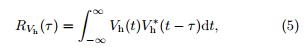
The wind energy spectra are used to characterize the variation of the wind energy density with frequency, and they are considered to be related to various weather systems. 2. 2 Turbulence spectrum analysis
Irregular fluctuation is the basic characteristicof turbulence. Horizontal wind can be calculated asVh =  h + u', where his the mean wind and u'isthe fluctuation. The Fourier transform of the autocorrelation function of u'is the turbulent energy spectraldensity .
According to Kolmogorov's theory(Kolmogorov, 1941a, b), the inertial sub-range is a turbulence regionwhere the Reynolds number is large enough to meetlocal homogeneous isotropic conditions, so its turbulence characteristics only depend on the dissipationrate. The energy spectral function is defined by
where k is the wavenumber, ε is the turbulence dissipation rate, and C is a constant. The function iscalled the "-5/3 law. " The inertial sub-range of theturbulence energy spectrum can also be expressed byfrequency(Sheng et al., 2003):where S(f)is the turbulence spectrum density . Theturbulence spectrum analysis using wind tower observations shows that the slope of the turbulence spectrum at frequencies between 10-2 and 102is -5/3 inthe inertial sub-range(Bian et al., 2002).
Figure 1 shows the turbulence spectrum changeswith wave number(Tian et al., 2011). The spectrumcan be divided into five ranges: the dissipation range, the inertial sub-range, the energy range, the largestvortex range, and the large eddy range. The energyrange produces turbulent energy, which can neitherbe generated nor be dissipated but is transferred tosmaller scales of motion in the inertial sub-range orchanged into internal energy because of the viscosityof the fluid molecules in the dissipative range. In theinertial sub-range, the slope of the turbulence spectrum is -5/3, which is steeper than the slope in the energy range but shallower than in the dissipation range(Kaimal and Finnigan, 1994). The turbulence spectrum density is normalized as: S'u' = Su'/σ2u', where σ2u' expresses the variance of wind fluctuation.
 |
| Fig. 1. Turbulence spectrum changes with wavenumber. (From Tian et al., 2011) |
The average wind data are usually treated as themean wind for data collected over a short period. However, the mean wind for wind data collected over longperiods changes with time, and is called the trend. The fluctuation of the wind is obtained by using theleast-square curve fitting to calculate the trend and deduct it from the wind data. Figure 2 shows the turbulence spectrum with two different methods used forthe mean wind calculation. In Fig. 2a, the averagewind data are treated as the mean wind and in Fig. 2b the trend is calculated as the mean wind. The dataare on 23 June 2011. Figure 2b shows a more distinct28-h eddy energy .
 |
| Fig. 2. The turbulent spectra obtained with mean wind derived di®erently . (a)Average as mean wind and (b)trendas mean wind. |
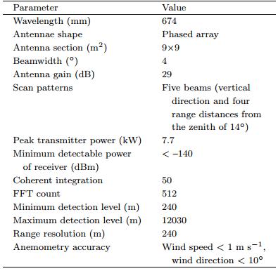
The horizontal wind-speed data used in the spectral analysis are obtained from CFL-08 tropospherewind profiler radar, which is located at Yanqing, Beijing(40. 45°N, 115. 96°E; 487. 90-m elev ation). Table 1summarizes the main properties of the radar. Rigorous calibration and st and ardization were carried outon the wind profile radar. Compared with air sounding, the accuracy of the wind profile radar correspondswith the specification. Deng et al. (2012)ev aluatedthe detection accuracy of the radar using observ ationsin 2010.
The wind profile radar provides horizontal windspeed data and signal-to-noise ratio(SNR), echo intensity, spectral width, and so on. The data were obtained from December 2010 to October 2012, at a sampling interv al of 6 min. Quality control was appliedas follows. Wind data that had an SNR of less than-15 dB were removed from the energy spectrum analysis because of their inaccuracy . Data series thathad five consecutive missing data points were rejected. When individual missing data occurred in the data sequence, neighboring data were used to fill the gap byusing linear interpolation.
According to the duration of different disastrousweather events, the data length chosen for cold windyweather and summer rainstorms is 7 days, while 3 daysis chosen for severe convective weather. The trend isidentified in the turbulence spectrum density calculation. Data used for the turbulence spectrum featuresof the stable weather analysis are detected every 6 minfor a period of 24 h. 4. Characteristics of turbulence spectrum athigh altitude
To examine the characteristics of the turbulencespectrum at high altitude, 10 sets of wind data under stable weather conditions are chosen. The dataperiod is 24 h and the frequency range is from 10-5to 10-2s-1. Figure 3 shows the normalized turbulence spectrum on 28 January 2011 at an altitude of1110 m. The abscissa is frequency and the ordinate isnormalized turbulence spectrum density . Logarithmiccoordinates have been used.
 |
| Fig. 3. Turbulence spectrum features on 28 January 2011 |
Figure 3 shows that the distribution of the turbulence spectrum is linear. By using least-square linear fitting, the turbulence spectrum density in the frequency range 2 × 10⁻⁵-10-3s-1can be expressed as
where a is the intercept of the abscissa, which is related to the turbulence dissipation rate; and b is theslope. The parameters of the turbulence spectrum forFig. 3 are a = 9 × 10⁻⁴, b = -0. 93, and the fittingrate is 0. 99.
Table 2 summarizes the values of a and b for theturbulence spectrum of the 10 sets of data under stable weather conditions at different heights: a variesfrom 4 × 10⁻⁴to 4 × 10⁻³ and b varies from -0. 82to -1. 04, which is less than the value(-5/3)in the inertial sub-range. The turbulence spectrum distributesin power in the frequency ranges of 2 × 10⁻⁵- 10-3s-1at heights between 1000 and 5000 m; b is less than-5/3, showing that the turbulence is in the energy region that is transiting to the inertial sub-range.
 |
The turbulence spectrum density of horizontalwind speed and its two orthogonal components u and v have been calculated. Figure 4 shows the turbulencespectrum of the horizontal wind speed, Vh, u, and v on1 December 2012 at an altitude of 1110 m. The resultsindicate that the three variables have a characteristicin common. The slope b is -0. 96, -0. 97, and -0. 97, inthe frequency range of 2×10⁻⁵-10-3s-1. It can thenbe concluded that the distribution of the turbulencespectrum in stable weather cases does not depend onthe wind direction.
 |
| Fig. 4. Turbulence spectrum features of di®erent variables at 1110-m height under stable weather on 1 December 2012. (a)u, (b)v, and (c)Vh. |
However, the situation is different for rainy days. Figure 5 shows the distributions of the turbulencespectrum for different variables at an altitude of 1110m in severe convective weather cases at 0000-2400 BT(Beijing Time)3 June 2012. The slope b is -0. 54, -0. 79, and -0. 76, which are quite different to those forstable weather cases.
 |
| Fig. 5. Turbulence spectrum features of di®erent variables at 1110-m height under rainy weather on 3 June 2012. (a)u, (b)v, and (c)Vh |
The wind energy spectrum in stable weather conditions is calculated as follows. The observ ations from0000 BT 5 to 2400 BT 11 December 2010, and 0000BT 3 to 2400 BT 5 July 2010 are chosen as typicalexamples of winter and summer weather conditions. Figure 6 shows that there is no peak during these periods, and the distribution of energy spectrum in thewhole frequency b and is relatively flat. The energyspectrum density decreases with increasing frequency . Figure 6 also shows that at the same height, the windenergy spectrum density in summer is nearly one order of magnitude smaller than in winter. The valuedecreases homogeneously with the reducing height inwinter, while in summer it is dense in the altituderange of 1000-2000 m. The distribution of the spectrum in the two seasons is similar, as is the normalizedturbulence spectrum in stable weather cases.
 |
| Fig. 6. Wind energy spectrum features for stable weather cases. (a)5-11 December 2012 and (b)3-5 July 2010. |
Table 3 gives a summary of the spectral density ofhorizontal wind at five heights in stable weather. Asthe height reduces from 5000 to 1000 m, the wind energy spectrum density decreases by one order of magnitude in winter, which is the same as that shown inFig. 6. In summer, the spectral density decreases byhalf. Overall, the spectral density change with heightis greater in winter than in summer.

The turbulence spectrum density accounting forthe proportion of wind energy spectrum density increases with frequency, as shown in Table 3. As theheight reduces, the ratio becomes greater as well, and this characteristic is more obvious in summer. 5. 2 Spectrum characteristics of cold windyweather
The data used in the spectrum analysis of coldwindy weather are from the Beijing wind profile radar. The sampling interv al is 30 min and the data periodis 7 days. On 11 November 2012, winds at level 5 or6 were observed in Beijing; in some local areas, windseven reached level 7, and then weakened to level 3 atnight with significant cooling. Figure 7a shows thehorizontal wind speed below the altitude of 5000 m, Fig. 7b shows the wind energy spectrum, and Fig. 7c shows the turbulence spectrum, for this cold windyweather. The five curves represent the spectrum density at 5070, 4110, 3150, 2190, and 1110 m.
 |
| Fig. 7. (a)Horizontal wind speed, (b)wind energy spectrum of horizontal wind, and (c)turbulent spectrum of horizontalwind, under cold windy weather during 8-14 November 2012. |
The different appearance of the wind energy spectrum for cold windy and stable weather in winter canbe seen in Fig. 7b. At the altitude range of 5070-2190m, the energy spectrum density only changes a little, while it decreases rapidly in the range of 2190-1110 m. This is different from the changes in stable weather. Inthe turbulence spectrum(Fig. 7c), compared with thestable weather, there is a clear peak at the frequency3. 0 × 10-5s-1. The intensity of the peak graduallydecreases from 5070 to 2190 m.
Table 4 gives the spectral density of horizontalwind at five heights in cold windy weather. Thereappears to be a transmission of the energy spectrumdensity from high to low altitudes. F rom 5070 to 2190m, the energy spectrum density decreases quickly and then increases slowly . In the peak area, the turbulencespectrum density accounting for the proportion of thewind energy spectrum density increases rapidly; thehigher the height, the higher the proportion. The ratios at the five heights are 22. 4%, 12. 8%, 9. 6%, 8. 8%, and 7. 3%, respectively .
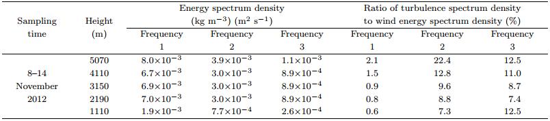
Table 4 and Fig. 7 show that there is a period of1. 5 days in cold windy weather where the wind energyspectrum from 5070 to 2190 m decreases quickly and then increases slowly . A strong wind shear caused theintense turbulence. The amplitude in the peak area athigh altitude is greater than at the lower levels. Thismay be due to the energy passing from the upper airto the lower levels. 5. 3 Spectrum characteristics of summer rainstorms
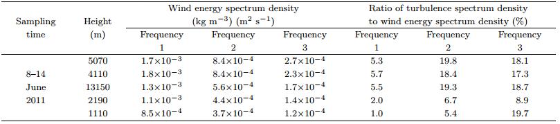
Compared with the stable weather, the turbulence spectrum during summer rainstorms has several peaks. This is the turbulence characteristics ofthe mesoscale rainstorm weather. On 23 June 2011, heavy rain fell in the Beijing area; total 24-h rainfall reached 241 mm. The rainstorm was sudden and intense. It had an uneven spatial distribution and significant mesoscale characteristics. The precipitation was concentrated in the period 16-19 h, withmany areas experiencing instantaneous hail. Figure 8a shows the horizontal wind speed below the altitude of 5000 m from 0000 BT 20 to 2400 BT 26June 2011. Figures 8b and 8c show the wind energyspectrum and the turbulence spectrum for this rainstorm.
 |
| Fig. 8. As in Fig. 7, but for summer rainstorms during 8-14 June 2011. |
The wind energy spectrum(Fig. 8b)shows thatthe amplitude decreases as the height reduces. In contrast to the spectrum in cold windy weather, the windenergy spectrum becomes more stable with height, and the slope of the wind energy spectrum decreases withdecreasing height. The spectrum density is only 20%of that in cold windy weather at the same altitude. There are 2-3 peaks at different heights in Fig. 8c. The peaks are located in the frequency range of 7 ×10⁻⁶-2 × 10⁻⁵s-1, and have a period of about 1 day . It can be seen that at 1110 m, there are two peakslocated at 5 × 10⁻⁶ and 2 × 10⁻⁵s-1, while there areno peaks at 2190 m.
Table 5 gives the spectral density of horizontalwind at five heights in the summer rainstorm case. The characteristic of spectral density changing withheight is similar to that in stable weather. The turbulence spectrum density accounting for the proportionof wind energy spectrum density significantly increasesin peak areas, which reflects that there are several disturbances in the rainstorm which occurred in the warmsector and there was no cold air at upper levels. Theoccurrence of the peaks may be because of the verticalmovement of precipitation clouds.
 |
On 3 June 2012, hailstorms, possibly due totrough-line activities, occurred in Beijing, with morethan 20 mm of precipitation. Figure 9a shows thehorizontal wind speed below the altitude of 5000m during 3-5 June 2012. Figure 9b shows thewind energy spectrum and Fig. 9c shows the turbulence spectrum for this severe convective weathercase.
 |
| Fig. 9. As in Fig. 7, but for the severe convective weather case during 3-5 June 2012. |
In Fig. 9b, the spectrum is smooth and there areno peaks. The amplitude is four times bigger thanin the summer rainstorm, and is close to that in coldwindy weather. F rom 5070 to 3150 m, the spectrumdensity decreases only a little, while it reduces rapidlybelow 3150 m, showing that the wind energy transmitsfaster at the lower level. The spectrum characteristicsare similar to those of cold windy weather because thetwo cases are both related to a cold front. The spectrum of turbulence has two peaks at all the heightsexcept 2190 m; one at a frequency of 2 × 10⁻⁵s-1 and the other at 6 × 10⁻⁵s-1. These peaks occurat about 13 and 9 h. The amplitude of the peaksis stronger at low altitude. The maximum amplitudeis at 3150 m and the minimum is at 5070 m, whichshows that the turbulence is more vigorous at 3000 m. This may be because of the activity of the trough-line. The amplitude at 1110 m is larger than that at 5070m, mainly because of the activity of turbulence in thewarm sector.
Table 6 is a summary of the spectral density ofhorizontal wind at five heights in this severe convective weather case. The spectral density decreases withdecreasing altitude. The amplitude of the spectrumat the same altitude and the same frequency in severe convective weather is larger than that in stableweather. The higher the frequency, the less the spectrum density, and the larger the turbulence spectrumdensity accounting for the proportion of the wind energy spectrum density, indicating that the energy inthe high energy scale at low frequency transmits tothe low energy scale at high frequency . In peak areas, the turbulence spectrum density accounting forthe proportion of the wind energy spectrum density islarger than other areas, especially at 3150 and 2190 m. This may be because of the intense vertical movementat the middle level.
 |
In this study, spectral analysis of wind profiling radar observ ations at heights of 1-5 km has beenmade. The wind energy and turbulence spectrum indifferent weather conditions shows different characteristics, which are helpful to the analysis and researchof weather systems.
Turbulence spectrum in stable weather conditionsat high altitude is expressed in powers in the frequencyrange 2 × 10⁻⁵-10-3s-1. The slope b is between-0. 82 and -1. 04, indicating that the turbulence is inthe transition zone from the energetic range to the inertial sub-range. Wind shear and convective activitymay enhance the turbulence.
The peaks seen in the turbulence spectrum showthe period of the weather system. Cold windy weatherappears at a period of 1. 5 days in the turbulence spectrum, and the amplitude at 5 km is the largest. Thewide-range summer rainstorm exhibits two or threepeaks in the spectrum over 15-20 h. In the severeconvective weather conditions there are two peaks at13 and 9 h.
Compared with stable weather, the turbulencespectrum density accounting for the proportion of thewind energy spectrum density increases rapidly, especially in peak areas, in severe weather conditions.
| [1] | Atkinoon, B. W., 1981: Mesoscale Atmospheric Circulations. Academic Press, 495 pp. |
| [2] | Bian Jianchun, Qiao Jinsong, and Lu Daren, 2002: Laboratory for middle atmosphere and global environment observation. Chinese J. Atmos. Sci., 26, 474-480. (in Chinese) |
| [3] | Bowne, N. E., and J. T. Ball, 1970: Observational comparison of rural and urban boundary layer turbulence. J. Appl. Meteor., 9, 862-873. |
| [4] | Chellali, F., A. Khellaf, and B. Adel, 2010: Application of time-frequency representation in the study of the cyclical behavior of wind speed in Algeria: Wavelet transform. Stochastic Environmental Research and Risk Assessment, 24, 1233-1239. |
| [5] | Deng Chuang, Ruan Zheng, Wei Ming, et al., 2012: The evaluation of wind measurement accuracy by wind profile radar. J. Appl. Meteor. Sci., 23, 523-533. (in Chinese) |
| [6] | Endlich, R. M., R. C. Singleton, and J. W. Kaufman, 1969: Spectral analysis of detailed vertical wind speed profiles. J. Atmos. Sci., 26, 1030-1041. |
| [7] | Griffith, H. L., H. A. Panofsky, and I. van der Hoven., 1956: Power-spectrum analysis over large ranges of frequency. J. Atmos. Sci., 13, 279-282. |
| [8] | Højstrup, J., 1981: A simple model for the adjustment of velocity spectra in unstable conditions downstream of an abrupt change in roughness and heat flux. Bound.-Layer Meteor., 21, 341-356. |
| [9] | Kaimal, J. C., J. C. Wyngaard, Y. Izumi, et al, 1972: Spectral characteristics of surface layer turbulence. Quart. J. Roy. Meteor. Soc., 98, 563-589. |
| [10] | —-, and J. J. Finnigan, 1994: Atmospheric Boundary Layer Flows: Their Structure and Measurement. Oxford University Press, 1-279. |
| [11] | Kolmogorov, A. N., 1941a: The local structure of turbu-lence in incompressible viscous fluid for very large Reynolds number. Math. Phys. Sci., 434, 9-13. |
| [12] | —-, 1941b: Dissipation of energy in the locally isotropic turbulence. Math. Phys. Sci., 434, 15-17. |
| [13] | Liu Shuyuan, Zheng Yongguang, and Tao Zuyu, 2003: The analysis of the relationship between pulse of land heavy rain using wind profiler data. J. Trop. Meteor., 19, 285-290. (in Chinese) |
| [14] | Liu Xiaohong and Hong Zhongxiang, 1996: A study of the structure of a strong wind event in the atmospheric boundary layer in Belting area. Scientia Meteor. Sinica, 20, 223-228. (in Chinese) |
| [15] | Luo Jianyuan and Zhu Ruizhao, 1993: The analysis of wind spectrum characteristics in surface layer in Badaling area of Beijing. Acta Energiae Solaris Sinica, 14, 279-287. (in Chinese) |
| [16] | Panofsky, H. A., 1955: Meteorological applications of power—Spectrum analysis. Bull. Amer. Mcteor. Soc., 36, 163-166. |
| [17] | —-, D. Larko, R. Lipschutz, et al., 1982: Spectra of velocity components over complex terrain. Quart. J. Roy. Meteor. Soc., 108, 215-230. |
| [18] | Sheng Peixuan, Mao Jietai, Li Jianguo, et al., 2003: Atmospheric Physics. Beijing University Press, Beijing, 227-228. (in Chinese) |
| [19] | Sun Aidong and Xu Yumao, 1997: Spectral characteristic and multi-scale analysis of a wet cold front in boundary-layer atmosphere. Scientia Atmos. Sinica, 17, 18-27. (in Chinese) |
| [20] | Sun Jisun, He Na, Wang Guorong, et al., 2012: Preliminary analysis on synoptic configuration evolvement and mechanism of a torrential rain occurring in Beijing on 21 July 2012. Torrential Rain and Disasters, 31, 218-225. (in Chinese) |
| [21] | Tian Yuji, Yang Qingshan, Yang Na, et al., 2011: Beijing meteorological tower statistical model of turbulent wind velocity spectrum. Scientia Sinica (Technologica), 41, 1460-1468. (in Chinese) |
| [22] | Van der Hoven, I., 1957: Power spectrum of horizontal wind speed in the frequency range from 0. 0007 to 900 cycles per hour. J. Meteor., 14, 160-164. |
| [23] | Wang Hua, Sun Jisong, and Li Jin, 2007: A comparative analysis on two severe hail events in Beijing urban district in 2005. Meteor. Mon., 33, 49-56. (in Chinese) |
| [24] | Wang Xinyan and Mao Jietai, 2004: The wavelet application in the research of mesoscale convective activity features. J. Trop. Meteor., 20, 549-560. (in Chinese) |
| [25] | Wei Fengying and Zhang Ting, 2009: Frequency distribution of drought intensity in Northeast China and relevant circulation background. Journal of Natural Disasters, 18, 1-7. (in Chinese) |
| [26] | Yu Xiaoding, 2012: Investigation of Beijing extreme flooding event on 21 July 2012. Meteor. Mon., 38, 1313-1329. (in Chinese) |
| [27] | Zhang Xiaoping, Lü Naiping, and Zhou Mingyu, 1987: The characteristics of vertical distribution of lowfrequency spectra for horizontal wind velocity in the atmospheric boundary layer. Chinese J. Atmos. Sci., 11, 31-39. (in Chinese) |
| [28] | Zhao Deshan, Wang Lizhi, and Hong Zhongxiang, 1982: Analysis on the structure of gust in boundary layer when a cold front passing. Chinese J. Atmos. Sci.,6, 324-332. (in Chinese) |