 2014, Vol. 28
The Chinese Meteorological Society
Article Information
- QIN Yanyan, GONG Jiandong, LI Zechun, SHENG Rifeng. 2014.
- Assimilation of Doppler Radar Observations with an Ensemble Square Root Filter:A Squall Line Case Study
- J. Meteor. Res., 28(2): 230-251
- http://dx.doi.org/10.1007/s13351-014-2046-6
Article History
- Received October 23, 2013;
- in final form January 12, 2014


2 Key Laboratory of Research on Marine Hazards Forecasting, National Marine Environmental Forecast Center, Beijing 100081;
3 Center for Numerical Weather Prediction, CMA, Beijing 100081;
4 National Meteorological Center, CMA, Beijing 100081;
5 Weather Modification Office of People's Government of Shandong, Jinan 250031
Numerical weather prediction(NWP)is an ini-tial and boundary condition problem. Accurate and balanced initial estimate of the atmospheric state isessential to the improvement of the NWP. With highspatial and temporal resolutions, Doppler radar dataare increasingly used to initialize the convective-scaleNWP, which plays a key role in improving the accuracyof early warning of disastrous weather on convectivescale. With establishment of the NEXRAD networkin China, there has been a rapid growth in the radardetection capability, data coverage, and data quality, which provides advantageous conditions for assimila-tion of radar data. The continuous development ofdata assimilation techniques and computing power inrecent years makes it possible to assimilate Dopplerradar data in high-resolution nonhydrostatic numeri-cal models.
The way of assimilating radar data mainly in-cludes thermodynamic retrieval(Gal-Chen, 1978; Hane and Ray, 1985), thermodynamic initialization(Lin et al., 1993; Xue et al., 1998; Zhang et al., 1998), nudging(Jones and Macpherson, 1997), three- or four-dimensional variational method(Sun and Crook, 1997; Xu et al., 2004; Yang Yanrong et al., 2008; Yang Yi et al., 2008; Xu et al., 2012), and Ensemble KalmanFilter(EnKF). EnKF is based on the Monte Carleidea, which utilizes a group of short-term ensembleforecasts to estimate the background error covari-ance. EnKF has been implemented in various atmo-spheric and oceanic models due to its advantages offlow-dependent background error covariance, nonlin-ear model and observation operator, no need for tan-gent linear and adjoint models, and easy paralleliza-tion(e. g., Yang et al., 2011). Since first introducedinto the geophysical field by Evensen(1994), EnKFhas become one of the most promising assimilationmethods. In recent years, considerable progress hasbeen made in exploring the potential of using EnKF toassimilate radar data on convective scale. As for simu-lated radar data assimilation, many studies focused onanalyses of flow field and thermodynamic and micro-physical fields through the observing system simula-tion experiments(OSSEs). These experimental stud-ies have demonstrated the feasibility and e®ectivenessof EnKF on storm scales(Snyder and Zhang, 2003; Zhang et al., 2004; Tong and Xue, 2005; Xu et al., 2006; Xue et al., 2006; Qin et al., 2012; Xu et al., 2012; Xue and Dong, 2013). However, there are fewsuch kind of studies conducted in China.
As for real radar data assimilation, Dowell et al. (2004)explored for the first time the feasibility of usingan EnKF on storm scale. In their study, 10 successivevolumes of a single radar radial velocity and reflectiv-ity observations over a period of 47 min were assimi-lated into a three-dimensional warm cloud model de-veloped by Sun and Crook(1997)by using an Ensem-ble Square Root Filter(EnSRF). Retrievals of windfields were generally correct, while the low-level coldpool was too strong compared with the observation, probably due to model errors and observational limita-tions. Xu et al. (2006)used the same model to assim-ilate six successive volumes of radial velocity and rainwater retrieved from reflectivity of Yichang-Jingzhoudual Doppler radar. Their study shows that by us-ing the EnKF technique, the wind fields together withthermodynamic and microphysical fields of a convec-tive heavy rainfall system can be well retrieved. How-ever, the model used in the above studies is a warmcloud model, which does not include the ice micro-physics. Only rain water mixing ratio is updated inthe analysis, while the retrieval of ice-phase hydrome-teor fields is not included. The ice-phase hydrometeorsactually exist and play an important role in exuberantconvective cells(Hu et al., 1998). In addition, pre-vious studies assimilating real radar data with EnKFonly focus on the accuracy of retrieved fields, insteadof assessing the performance of forecasts initialized byanalyzed fields.
In this study, the performance of the EnSRF tech-nique is examined by applying it to the assimilationof real radar data during a squall line event on 12July 2005 in midwest of Sh and ong Province using theWeather Research and Forecasting(WRF)model witha complex multiclass ice microphysics scheme. A de-terministic prediction is also made using the ensemblemean of the third assimilation cycle as the initial con-dition. All variables including ice species are updatedin our analysis, and we concern not only the accuracyof retrieved state of the storm, but also the accuracyof prediction from this retrieved state. 2. EnSRF technique and assimilation system
In the st and ard EnKF formulation, observationsare treated as r and om variables that are subjectto added perturbations(Houtekamer and Mitchell, 1998), which will cause sampling errors associatedwith the use of perturbed observations. The EnSRFmethod, which does not perturb observations, is de-signed by Whitaker and Hamill(2002)to avoid theissue. They demonstrated that EnSRF produces ananalysis ensemble with mean error lower than that ofEnKF for the same ensemble size. The comparisonwas done in a Lorenz model and a two-level idealizedgeneral circulation model(GCM).
Similar to other ensemble-based Kalman filters, the EnSRF algorithm has two steps: integration and analysis. At the integration step, a set of short-termensemble forecasts are performed; while at the analy-sis step, background error covariance is estimated fromthis ensemble, and then the ensemble is updated. Theupdated ensemble is integrated forward until new ob-servations are available again and the sequential dataassimilation cycle is repeated. EnSRF is distinctivein that the ensemble mean( a) and the deviations ofensemble members from the mean(x'a)are updatedseparately. Under the assumption of independence ofobservations, the order in which we assimilate them isirrelevant. Observations are analyzed serially, until allthe observations are assimilated.
The analysis equation for ensemble mean state is:
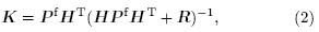
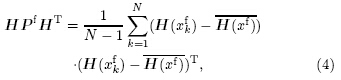
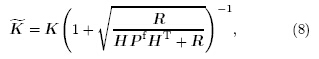
in which the superscripts a and f denote analysis and forecast, respectively; H is observation operator thatprojects model state to observation yo, and K is theKalman gain matrix:where R is observation error covariance matrix, H isthe Jacobean matrix of H, and Pf is prior error co-variance matrix which in practice does not need to becalculated explicitly in the EnSRF algorithm, whilethe background error covariance PfHT and HPfHTare estimated according towhere k represents the kth ensemble member, and Nis the ensemble size.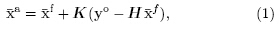
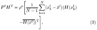
Sampling errors due to limited ensemble size willcause unreliable background error correlations be-tween analysis points and observations at large dis-tance. In our study, we settle this problem by us-ing a Schur product(Houtekamer and Mitchell, 2001), which is often called "covariance localization". In Eq. (3), Po donates a Schur product of a quasi-Gaussiancorrelation matrix with the background error covari-ance matrix, and the correlation function ½ is definedas a fifth-order piecewise rational function proposedby Gaspari and Cohn(1999)as follows,
where c is a pre-specified critical distance, and r isthe distance between observations and analysis gridpoints:In the EnSRF algorithm, observations are as-similated one at a time, HPfHT and R becomescalars for one observation, and thus the calculationof(HPfHT + R)-1 becomes a scalar inversion. Theimplementation of sequential assimilation of observa-tions and covariance localization settles the problemof huge computational costs in matrix inversion whencalculating K, which makes the EnKF algorithm fea-sible for large systems.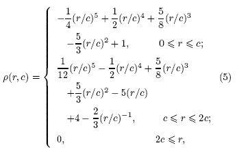
The deviation of kth ensemble member from themean is updated by:
where and γ is a covariance inflation factor, which is used toadjust the spread of ensemble, thus relieving the filterdivergence caused by sampling errors in the estimationof Pf due to small ensemble sizes. Ensemble varianceshould represent the statistics of the error of the en-semble mean forecast. Small ensemble spread tends tomake the analysis algorithm reject observations; oth-erwise, the analysis algorithm rejects background. Inpractice, the deviation of each member from the en-semble mean is multiplied by this inflation factor be-fore the first observation is assimilated.
Both radial velocity and reflectivity are assimi-lated in this study. The observation operator for ra-dial velocity and reflectivity are the same as that in Tong and Xue(2005). Vr is calculated from
where Vr is the observation of radar radial velocity, α and β are elevation angle and azimuth angle of radarbeams respectively, and u; v, and w are the three windcomponents output from the WRF model.
The observation operator for reflectivity is:
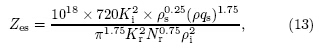
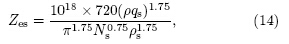
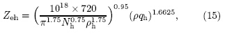
where Ze is reflectivity factor in unit of mm6 m-3, and Z is its logarithm in unit of dBZ. Ze is estimated asthe sum of contributions from three categories of hy-drometeors: reflectivity from rain Zer, snow Zes, and hail Zeh, i. e., The computation of each component of reflectivity isbased on Smith et al. (1975) and Lin et al. (1983)asfollows. Reflectivity for rain isreflectivity for dry snow when temperature is below0℃ iswhile reflectivity for wet snow when temperature isabove 0℃ is and reflectivity for hail iswhere ρ is air density, specifically, ½r = 1000 kg m-3is the density of rainwater, ρs = 917 kg m-3 is thedensity of snow, ρi = 913 kg m-3 is the density ofice, and ρh = 913 kg m-3 is the density of hail; qr, qs, and qh are the mixing ratios for rain, snow, and hail, respectively; Nr = 8. 0 × 10-6 m-4, Ns = 3. 0 ×10-6 m-4, and Nh = 4. 0 × 10-6 m-4, which are theintercept parameters in the assumed Marshall-Palmerexponential drop size distributions for rain, snow, and hail respectively. Ki2= 0. 176 and Kr2= 0. 93 are thedielectric factors for ice and water, respectively. The feasibility of this assimilation system hasbeen tested by Qin et al. (2012)through OSSEs. Inthis study, the e®ect of assimilating real radar datais explored by applying the assimilation system to asquall line case study. 3. Description of the case3.1 Overview of the event


A squall line hit midwest Sh and ong Province on12 July 2005 under the synoptic environment of atransverse(east-west oriented)trough related to anortheast vortex being transformed into a north-southoriented trough. From 1100 to 1500 BT(BeijingTime), thunder storm, strong winds, and hail oc-curred in succession at Gaotang, Yucheng, Qihe, Ji-nan, Laiwu, Boshan, and Yiyuan stations of Shan-dong Province, and hail occurred mainly at Gaotang, Yucheng, Laiwu, and Yiyuan stations. The diame-ter of hail observed at Xinzhuang town of Laiwu citywas about 25 mm, and the maximum accumulatedhail reached 30-40 mm. Strong wind was observedin the region between Jinan and Yiyuan stations, withwind speed above 20 m s-1. Instantaneous wind speedreached 22. 4 m s-1 at Laiwu station at 1330 BT, and 29. 2 m s-1 at Yiyuan station at 1440 BT. This squallline has caused enormous economic loss in Sh and ongProvince. 3.2 Synoptic environment of the event
A vortex stayed over Northeast China from 8 to11 July, behind which a ridge strengthened and de-veloped northeastward. The vortex center then weak-ened and moved southward, with a transverse troughgenerated to its west. At 0800 BT 12 July, the vor-tex disappeared, accompanied with an anticlockwiseturning of the transverse trough. The prevailing winddirection at 500(Fig. 1a) and 700 hPa(figure omit-ted)was west-northwest over Sh and ong Province. At850 hPa(Fig. 1b) and below, a cyclonic shear lay overthe boarder of Hebei, Henan, and Sh and ong provinces, and the wind in midwest Sh and ong Province was weaksouthwesterly. The sounding at Zhangqiu station re-vealed that the 24-h temperature tendency at 0800 BT12 July was +2℃ at 850 hPa and -1 at 500 and 700hPa. This indicated that temperature increased ob-viously in the low troposphere, while cold air invadedthe mid-upper troposphere. In such a synoptic envi-ronment of the transverse trough being transformedinto a north-south one, the upper-level cold air wentdown and unstable stratification formed, inducing se-vere convective weather.
 |
| Fig. 1. Synoptic charts of(a)500 and (b)850 hPa at 0800 BT 12 July 2005. |
The squall line system moved from west to eastin midwest Sh and ong Province, and precipitation de-veloped along with it. Thunder shower less than 1mm occurred at 0800 BT 12 July in Northwest Shan-dong. The intensity and range of precipitation in-creased from 1200 to 1700 BT, and local precipitationincreased obviously. Rainfall intensity was 18 mm h-1at 1200 BT, and reached its maximum value of 43 mmh-1 at 1400 BT around Tai0an station, then weakenedto be 12 mm h-1 at 1600 BT around Yiyuan station. The precipitation abated to a general thunder showerat 1800 BT, and located mainly in the area of highsurface pressure. From 1800 to 2000 BT, precipita-tion continued to abate and gradually moved out ofSh and ong Province. 3.4 Radar observations
This mesoscale convective event was observed bythe CINRAD-SA Doppler radar in Qihe county ofJinan area(with radar antenna located at 36. 81°N, 116. 78°E, and 72. 9 m above sea level). The volumescan mode of the radar was VCP 21, of which theradar completed 9 elevations ranging from 0. 5° to19. 5° within 5-6 min. The radar gave observations ofreflectivity and radial velocity at each elevation, withmaximum detection radius of 460 and 230 km respec-tively, and resolutions of 250-m gate spacing and 1°azimuth respectively.
The evolution of composite reflectivity fieldshowed that the convective storm was initiated in theearly morning of 12 July near Yangquan city of ShanxiProvince. It developed eastward, and then two con-vective cells formed at 1056 BT in Xiajin county ofDezhou area(with maximum reflectivity of 55 dBZ and echo top at 12 km) and Qinghe county of HebeiProvince. They strengthened and evolved end to endgradually(Fig. 2a). An intense echo emerged nearGaotang station at 1126 BT(Fig. 2a) and developedsouthward, while a bow-shaped echo began to developin the western portion of the echo with maximum re-flectivity of 68 dBZ at 1202 BT. At the same time, aclear outflow boundary occurred behind the new bornechoes, and convective cells formed continuously onthe tail of it. The bow-shaped echo formed at 1232BT(Fig. 2c)with convergence of the new-born con-vective echo and the former echo, and an echo notchappeared on the back side of the bow's head, indi-cating a strong inflow on the back side of the bowecho. During 1100-1300 BT, with the bow echo pass-ing through, hail occurred in Gaotang and Yucheng, and thunderstorm gale occurred in Liaocheng and Ji-nan, with gust velocity of 18 m s-1. The bow echomoved southward and converged with new-born cells, and began to weaken after 1357 BT. An isolated mas-sive echo formed near Laiwu at 1238 BT, strengthenedwhile moving northeastward, and reached maximumreflectivity of 63 dBZ at 1321 BT. It then began toweaken and dissipate at 1609 BT. At the same time, new convective cells developed on the right side of theaforementioned echo, and developed into a supercellat 1339 BT, with maximum reflectivity of 67 dBZ and echo top of 13 km. A®ected by this supercell, hail and thunderstorm gale hit Laiwu. The bow echo evolvedinto a comma cloud during 1403-1421 BT, and movedsoutheastward over Sh and ong Province from then on, and gradually dissipated.
 |
| Fig. 2. Compound radar re°ectivity at Jinan at(a)1126, (b)1202, (c)1232, and (d)1321 BT 12 July 2005. |
This study includes two experiments as shown inFig. 3: the assimilation experiment of real radar data and the control run without data assimilation. Bothexperiments begin at 0800 BT 12 July 2005, with inte-gration time of 12 h that covers the whole developmentof the squall line event. The NCEP global reanalysisdata are used as initial and boundary conditions. Inthe assimilation experiment, the model first integrates1 h before the first assimilation at 0900 BT in orderto develop a flow-dependent background error covari-ance that corresponds to the synoptic process. Then, real radar observations are assimilated every 30 minat 0930 and 1000 BT, and a deterministic forecast of10 h is followed thereafter, initialized by the ensemblemean analysis of the 3rd assimilation cycle.
 |
| Fig. 3. Flow chart of the experiment scheme. |
In this study, version 3. 2 of WRF, a fully com-pressible nonhydrostatic mesoscale model, with itsAdvanced Research WRF dynamic core, is used. Ithas six prognostic equations and one static diagnos-tic equation. The prognostic variables include threevelocity components, perturbation potential tempera-ture, perturbation geopotential, and perturbation sur-face pressure of dry air, and optional prognostic vari-ables such as mixing ratios for water vapor, cloud wa-ter, rain, ice, snow, and graupel. Two model domainswith two-way nesting are employed. The coarse do-main has 201 × 201 grid points and a grid space of 9km, and the integration time step is 60 s. The innerdomain has 280 × 247 grid points and a grid spaceof 3 km. Both model domains have 28 vertical layers, and the model top is set at 50 hPa. The cumulus pa-rameterization scheme for coarse domain is the Kain-Fritsch scheme(Kain and Fritsch, 1990, 1993). Nocumulus parameterization scheme is used in the innerdomain. The microphysics scheme is WSM6(WRFSingle-Moment 6-class)scheme(Hong et al., 2004)forboth domains, from which mixing ratios of water va-por, cloud water, rain, ice, snow, and graupel can beoutput. The NCEP final FNL analysis data on a 1°×1° resolution are used to create the initial and bound-ary conditions. 4.3 Assimilation parameters
Both radar reflectivity and radial velocity are as-similated and all variables are updated in this study. Data assimilation is performed only for the inner do-main. The cuto® radii of covariance localization are 10model grids horizontally and 5 model grids vertically, and the covariance inflation factor is set to 2. 0. Ob-servation operators are given by Eqs. (9)-(15). Lim-ited by computer resources, the ensemble size is set to20. Encouraged by our previous results of OSSEs thatmodel storm can be reasonably rebuilt after three as-similation cycles(Qin et al., 2012), three assimilationcycles are performed in this study. 4.4 Ensemble initial perturbations
The initial ensemble is generated by theWRF three-dimensional variational data assimilation(3DVAR)using the cv3 background error covarianceoption, same as Zhang et al. (2006)in which they used3DVAR of the nonhydrostatic fifth-generation Penn-sylvania State University-National Center for Atmo-spheric Research Mesoscale Model(MM5)to generateinitial ensemble for their EnKF system. Firstly, 20r and om perturbations of stream function, namely con-trol vectors, which are consistent with the backgrounderror covariance used by the WRF 3DVAR system, aregenerated, and then transformed back to model spacevia a recursive filter in horizontal direction, an em-pirical orthogonal function(EOF)transform in verti-cal direction, and physical transformation. The initialperturbation is largely geostrophic balanced, which in-cludes horizontal wind components, potential temper-ature, and mixing ratio for water vapor. Other prog-nostic variables such as vertical velocity and mixingratios for cloud water, rain, ice, snow, and graupel arenot perturbed. 5. Preprocessing of radar data5.1 Quality control
Preprocessing and quality control of radar dataare performed as follows:
(1)Ground clutter is identified and removed byanalyzing the three-dimensional structure characteris-tics of radar reflectivity. Ground clutter rejection isimplemented by means of calculating horizontal tex-ture of reflectivity, vertical gradient of intensity, and the restrictive value of vertical gradient, and thengaps in precipitation echo areas potentially created bythe algorithm are filled by using the echo information(Xiao, 2007).
(2)Radar observations, radial velocity as well asreflectivity, are thinned to the resolution of 4 km in theradial direction, and the resolution after data thinningis almost the same as the model grid spacing.
(3)The observation errors of reflectivity and ra-dial velocity are assumed to be 5 dBZ and 3 m s-1respectively in this study. The observation will be dis-carded if the di®erence between observation and back-ground is larger than three times of the observationerror. 5.2 Observations to be assimilated
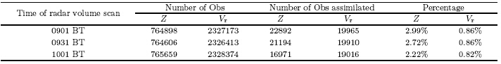
A significant amount of observations have beendiscarded after quality control and preprocessing(seeTable 1). Reflectivity data to be assimilated accountfor about 2%-3% of one volume scan, and radial ve-locity data to be assimilated only account for about1% of one volume scan. Corresponding to the timeof 3 assimilation cycles at 0900, 0930, and 1000 BT, the Doppler radar volume scans used in the currentstudy are at 0901, 0931, and 1001 BT. Figure 4 shows the observations to be assimilated in the firstassimilation cycle after preprocessing, in which obser-vations of di®erent heights are projected to a horizon-tal plane.
 |
| Fig. 4. Observations of(a)re°ectivity(dBZ) and (b)radial velocity(m s¡1)to be assimilated in the ¯rst assimilationcycle. |
Table 1 shows the number of observations before and after data preprocessing used in the three assimi-lation cycles, and the percentage of observations to beassimilated in the volume scan.
In this section, comparisons of wind fields, hy-drometeor fields, and precipitation are made betweenforecasts of control run, ensemble mean forecasts, en-semble mean analyses of the assimilation experiment, and observations, so as to assess the performance ofthe EnSRF scheme in retrieving the dynamical and microphysical fields of the squall line case. 6.1.1 Wind fields
The performance of the EnSRF scheme in ana-lyzing the low-level horizontal wind field is assessedby comparisons between radial velocity observationsin plane position indicator(PPI)at 0. 5° elevation and wind fields of control run and assimilation experiment. During 0900-1000 BT 12 July, radial velocity north-west of the Jinan radar is departing from radar with amaximum value of 19 m s-1, and radial velocity south-east and south of the radar is orientating toward radar and is 5-10 m s-1. Thus, at low levels below 850 hPa, strong southeast wind prevails northwest of the radarin Qinghe, Xiajing, Linqing, and Wucheng areas, and weak southwest wind occurs southwest of the radar inYanggu area. Weak south wind occurs south of theradar near Dongping county, and over the boarder ofSh and ong and Hebei provinces there is a cyclonic windshear from southwest to southeast.
Radial velocity of ensemble mean analyses of thethree assimilation cycles can be calculated from theobservation operator for radial velocity(Eq. (9)), and the distribution of thus calculated radial velocity onthe fifth model level(about 900 hPa)are shown inFig. 6. It is seen by comparing Fig. 5 with Fig. 6 that radial velocity fields at 900 hPa from the ensem-ble mean analysis are basically in accordance with theobservations.
 |
| Fig. 5. Radial velocity PPI observations at 0. 5° elevation at(a)0901, (b)0931, and (c)1001 BT 12 July 2005. |
 |
| Fig. 6. Radial velocity at about 900 hPa calculated from the ensemble mean analysis at(a)0900, (b)0930, (c)1000BT 12 July 2005. The black dot denotes location of the Jinan radar. |
Figure 7 shows the horizontal wind vector at 900hPa from the control run, ensemble mean forecast, and ensemble mean analysis at 0930 BT 12 July 2005. Equivalent figures at 0900 and 1000 BT are omitted. It can be seen that, in the west and central parts ofSh and ong Province, the wind fields at 900 hPa of thecontrol run are smooth, weak, and southward, whichare inconsistent with the observations characterized bystrong southeast wind and a cyclonic shear at low lev-els in the northwest of Sh and ong. In contrast, theradial velocity fields from the ensemble mean anal-ysis are in good accordance with the observations, and radial velocity greater than 19 m s-1 departing fromthe radar can be seen around Qinghe, Xiajing, and Linqing areas in Fig. 6. An obvious wind shear ex-tending from south-southwest to southeast over theboarder of Sh and ong and Hebei provinces is seen in theensemble mean forecast and ensemble mean analysis at900 hPa, which is consistent with the low-level obser-vations. Moreover, after data assimilation, the southwind around Lingxian becomes stronger, and agreesbetter with observations. The low-level wind shear, strengthening southeast wind around Qinghe, Xiajing, and Linqing, together with strengthening south windaround Lingxian, cause a low-level wind convergencein Northwest Sh and ong, which all contribute to thegenerating of updraft by the model atmosphere, and this has made preparations for the advent of the sub-sequent convective weather.
 |
| Fig. 7. Horizontal wind vector at 900 hPa from(a)control run forecast, (b)ensemble mean forecast, and (c)ensemblemean analysis, of the second assimilation cycle at 0930 BT 12 July 2005. |
Through comparison between radial velocity cal-culated from control run and assimilation experiment, and radial velocity observations at 1. 5° and 2. 4° eleva-tions, the analyzed upper-level wind fields after assim-ilation are closer to the observations than that of thecontrol run. From radial velocity PPI observations at1. 5° and 2. 4° elevations at 0901, 0931, and 1001 BT, it can be seen that at 500 hPa, a strong northwest airflow appears in the northwest of Sh and ong Province and south of Hebei Province, and a weak west south-west air flow shows up in the central and southwestof Sh and ong Province, and there is a trough orientedfrom northwest to southwest in the upper air abovethe radar. In comparison with the radial velocitycalculated from ensemble mean analysis of the 10thmodel level(about 550 hPa), it is found that, afterassimilation, the radial velocity in upper air is in goodaccordance with the observation, with radial velocityof 19 m s-1 orientating toward radar in the northwest and southwest of the radar, and radial velocity depart-ing from radar in the east of the radar.
A comparison of horizontal wind fields at 500 hPaat 0900, 0930, and 1000 BT from the control run, ensemble mean forecast, and ensemble mean analy-sis shows that although the control run produces thetrough at 500 hPa, the flow field is too smooth to de-scribe the strong northwest air flow along the Dezhou, Hengshui, Xinji, and Wuji areas; while the northwestair flow is strengthened in the aforementioned areaafter assimilation, and the wind fields in Hejian and Xianxian of Hebei Province have also been better sim-ulated.
We now examine the performance of the EnSRFin retrieving the vertical wind field. As analyzedabove, the low-level horizontal wind fields convergearound 37. 2°N during 0900-1000 BT, and there oc-cur vigorous convective clouds and strong vertical mo-tion there. A cross-section of velocity, temperature, and total mixing ratio of hydrometeors(sum of mixing ratio for cloud water, rain, ice, snow, and graupel)along 37. 2°N is plotted for the control run forecast, en-semble mean forecast, and ensemble mean analysis at0900, 0930, and 1000 BT. It can be seen that, the in-crease of vertical velocity from the control run is slow and weak and does not reach 1 m s-1 until 1000 BT, and the total mixing ratio of hydrometeors from thecontrol run is also very small(Fig. 8b). Such weakvertical motion and low content of hydrometeors donot accord with observation of the severe convectivesystem. By contrast, in the assimilation experiment, the upward velocity before the 1st assimilation cycledoes not reach 0. 5 m s-1(Fig. 8c), but it increasesobviously to 4 m s-1 after the 1st assimilation cycle(Fig. 8d). Hydrometeors develop quickly along withthe upward motion through model dynamics, and havea good correspondence in position with the upwardflow. Vertical motion weakens at 1000 BT comparedwith that at 0930 BT, which is also in agreement withthe observation that the convective clouds are weak-ening during this period.
 |
| Fig. 8. Longitude-height cross-sections of vertical velocity(shaded), temperature(green contour), and total mixing ratioof hydrometeors(black contour; g kg-1)along 37. 2°N of(a)forecast of control run at 0900 BT, (b)forecast of controlrun at 1000 BT, (c)ensemble mean forecast at 0900 BT, and (d)ensemble mean analysis of the second assimilation cycleat 0900 BT 12 July 2005. |
As can be seen from the above, by assimilationof radar data using EnSRF, detailed characteristics ofwind fields, such as cyclonic shear at the low level, the high velocity region, and low-level wind conver-gence in Xiajing area have been accurately retrieved. Moreover, the vertical motion has also been strength-ened, which helps development of the convection. Thewind fields after assimilation of radar data agree bet-ter with the observations. 6.1.2 Microphysical fields
It can be seen from reflectivity PPI observationsat 0. 5°(Fig. 9) and 1. 5° elevations(figure omitted)that convective cells develop northwest of the radarwith maximum reflectivity of 60 dBZ, and weakengradually from 0900 to 1000 BT. The height of thisecho is about 2-5. 5 km estimated from radial distance and elevation of the echo. There should be a region ofhigh hydrometeor content between 700 and 500 hPaaccordingly. In the control run, the convection hasnot developed yet due to model spin-up. Hydrome-teors only appear in local areas with a small value ofless than 1. 0 g kg-1 at 500 and 700 hPa(Figs. 10a1-c1 for 500 hPa; the 700-hPa figure is omitted). Bycontrast, in the assimilation experiment, informationof hydrometeors is added into the analyzed field, and hydrometeor field has been greatly improved. The to-tal mixing ratio of hydrometeors exceeds 1. 0 g kg-1in most areas, and in better accordance with the ob-servations in the northwest of Sh and ong at 500 and 700 hPa(Figs. 10a2-c2).
 |
| Fig. 9. Reflectivity PPI observations at 0. 5° elevation at(a)0901, (b)0931, and (c)1001 BT 12 July 2005. |
 |
| Fig. 10. Forecast total mixing ratio of hydrometeors(g kg-1)at 500 hPa from the control run at(a1)0900, (b1)0930, and (c1)1000 BT, and ensemble mean analysis at(a2)0900, (b2)0930, and (c2)1000 BT 12 July 2005. |
Encouraged by accurate retrieval of dynamic and thermal fields of the squall line with the use of the as-similation scheme, a deterministic forecast to 2000 BTis made from the ensemble mean analysis of the 3rdassimilation cycle. In this section, this forecast is as-sessed through comparison with the forecast from thecontrol run and the observations. 6.2.1 Microphysical fields
Forecasts of microphysical fields from ensemblemean analysis will be verified by a comparison be-tween forecast reflectivity and observed reflectivity. Asshown in Fig. 11a, a bow-shaped echo lies south of Ji-nan at 1. 5° elevation, with a radial distance of about150 km from the radar and maximum reflectivity of50 dBZ. It is estimated that the height of the echo is4 km(600 hPa or so). The forecast reflectivity by thecontrol run is much larger than the observation in awhole, with maximum values of basically 55-60 dBZ(Fig. 11b); while the forecast reflectivity by ensemblemean analysis has a closer distribution to the obser-vation in the location of strong and weak echoes, and the value of reflectivity is also closer to the observation(Fig. 11c). Comparison of forecast reflectivity fieldsfrom both the control run and the assimilation experi-ment at 1400 BT with the observations shows that theforecast from ensemble mean analysis still has encour-aging e®ects after a 4-h integration(figures omitted).
 |
| Fig. 11. (a)Reflectivity PPI observation at 1. 5° elevation at 1303 BT. Forecast re°ectivity(dBZ)at 600 hPa from(b)control run and (c)ensemble mean analysis of the assimilation experiment at 1300 BT 12 July 2005. |
The forecast accuracy of ensemble mean analy-sis gradually decreases after model integration for 5 h, as indicated by faster development and quicker move-ment of the simulated squall line than the observed. This may be attributed to a relatively stronger westwind that is assimilated into the model. But the forecast from ensemble mean analysis is still closer to ob-servation than that from the control run. After in-tegration of 8 h, neither the forecast from ensemblemean analysis nor the forecast from the control run isin agreement with the observation.
Figure 12 shows the reflectivity PPI observationat 1.5° elevation at 1409 BT, and its vertical cross-section along line AB, located at about 35. 7°N, and Fig. 13 is the vertical cross-sections of forecast re-flectivity along 35. 7°N from both the control run and the ensemble mean analysis. Figures 12 and 13 revealthat the squall line is well organized into a belt-shapedsystem and the forecast initiated from ensemble meananalysis has a better performance in describing such abelt-shaped arrangement of convective cells, as well asin forecasting the height and intensity of each convec-tive cell.
 |
| Fig. 12. (a)Reflectivity PPI observation at 1. 5° elevation and (b)cross-section of reflectivity along line AB at 1409BT 12 July 2005. |
 |
| Fig. 13. Longitude-height cross-section of forecast reflectivity(dBZ)along 35. 7°N from(a)control run and (b)ensemblemean analysis of the assimilation experiment at 1400 BT 12 July 2005. |
As shown by the visible cloud imagery fromthe Moderate Resolution Imaging Spectroradiometer(MODIS)at 1050 BT 12 July(Fig. 14), a small-scalebut deep cloud system developed in the west of Shan-dong Province, with a shallow cloud periphery. Thetotal hydrometeor at 500 hPa produced by the controlrun(Fig. 15a)is much less than the MODIS data, while the forecast hydrometeor field from the assimi-lation experiment(Fig. 15b)has a more reasonabledistribution and structure.
 |
| Fig. 14. Visible cloud imagery by MODIS at 1050 BT 12July 2005. |
 |
| Fig. 15. Total mixing ratio of hydrometeors(g kg-1)at 500 hPa from(a)control run and (b)ensemble mean analysisof the assimilation experiment at 1100 BT 12 July 2005. |
Figure 16 shows the horizontal wind field and to-tal mixing ratio of hydrometeors at 500 and 950 hPaafter 4-h integration initiated from ensemble meananalysis of the 3rd assimilation cycle. An obvious ver-tical wind shear appears, as indicated by red circlesin Fig. 16. The environment wind is mainly north-westerly and westerly above 850 hPa, and turns intoeast and south wind below 850 hPa. The shift of winddirection from the upper to the lower atmosphere canreach 90°-180°. Such a vertical wind shear conformsto the typical feature of the wind field and structure ofa convective storm, and is favorable for maintenance and development of the storm(Yu et al., 2006).
 |
| Fig. 16. Horizontal wind field(vector) and total mixing ratio of hydrometeors(shaded; g kg-1)by ensemble meananalysis at(a)500 and (b)950 hPa at 1400 BT 12 July 2005. |
As shown in Fig. 16b, at the leading edge of thestorm, there is an outflow region for downdraft, wherethe horizontal wind speed reaches 20 m s-1. Duringthe saturation-adiabatic subsidence of rain droplets, the air is dragged down and cooled due to the evapora-tion and melting. The cold downdraft spreads outwardnear the ground layer and forms a cold outflow. It thenconverges strongly with the southwesterly warm moistair at the leading edge of the storm and forms a gustfront, which is in accordance with the ground obser-vations of gale and temperature decrease at 1400 BT. The strong convergence and unstable energy aroundthe gust front drive continuous development of thestorm. The vertical cross-section along 35. 4°N of fore-cast total hydrometeor and temperature fields at 1400BT shows that there is a cold pool in the convectivecell near the boundary layer(figure omitted), whichis caused by cold downdraft of precipitation particles, and there is a warm region in the middle of the convec-tive cell, which might be caused by latent heat releaseof hydrometeors in that region, and corresponds tothe dynamic and thermal characteristics of convectivecells.
The above analysis has demonstrated that fore-cast of wind fields and storm structure initiated fromensemble mean analysis is consistent with the charac-ters of convective cells, and the distribution and collo-cation of dynamic and thermal fields are also reason-able. 6.2.3 Precipitation
As shown by Fig. 17, precipitation occurredin southeast of Hebei, north of Sh and ong, and overthe boarder of Hebei and Sh and ong provinces during0800-0900 BT, with hourly rainfall exceeding 30 mmin some places. The control run starts at 0800 BT, and does not produce precipitation after 1. 5-h integrationat 0930 BT due to model spin-up(Fig. 18a). Bycontrast, precipitation occurs quickly after 0. 5-h inte-gration at 0930 BT, when the model is initiated fromensemble mean analysis of the 1st assimilation cycleat 0900 BT(Fig. 18b). Compared to the observation, precipitation forecast over the boarder of Hebei and Sh and ong during 0900-0930 BT by the assimilationexperiment is basically correct. Although the amountof precipitation is a little bit larger, the precipitationarea is in good consistency with the observation. Byassimilation of radar data using EnSRF, the modelspin-up time has been shortened and forecast of pre-cipitation has been improved considerably.
 |
| Fig. 17. Hourly surface precipitation(mm)observation during(a)0800{0900 and (b)0900{1000 BT 12 July 2005. |
 |
| Fig. 18. Accumulated precipitation(mm)from(a)control run and (b)assimilation experiment during 0800{0930 BT12 July 2005. |
The accumulated precipitation observation in Fig. 19a indicates that the rain falls mainly in the midwestof Sh and ong Province, with a northwest-southeastbelt-shaped distribution and a maximum value exceed-ing 60 mm at 36. 3°N, 116. 8°E. Precipitation forecastby the control run is larger than that of observationin general, especially in the north of Sh and ong(Fig. 19c). But it is greatly improved in the assimilationexperiment, with a much closer intensity in the north and over the Sh and ong Peninsula and basically cor-rect location and intensity of precipitation near thesquall line. Moreover, the forecast precipitation overthe Sh and ong Peninsula and Rizhao area is also accu-rate(Fig. 19b).
 |
| Fig. 19. Accumulated precipitation(mm)of(a)observation, (b)forecast by the control run, and (c)forecast by theassimilation experiment during 0800{2000 BT 12 July 2005. |
This study explores the potential of using En-SRF to assimilate real radar data on convective scalethrough a squall line case study in midwest Sh and ongProvince by employing the WRF model. Assessmentis made using a variety of observations such as radardata, satellite data, and precipitation data. The ex-perimental results show that:
(1)The EnSRF system demonstrates greatpromise in assimilating real Doppler radar data toinitiate the convective squall line. Through radardata assimilation every 30 min, the convective-scaleinformation is added into the high-resolution nonhy-drostatic numerical model, and accurate and detailedstructures of wind field, such as low-level cyclonic windshear, severe wind region, and low-level wind conver-gence, can be analyzed e®ectively. Microphysical fieldscan also been retrieved accurately. The model spin-uptime has been shortened, and the forecast of precipi-tation has been improved accordingly.
(2)Deterministic forecast initiated with the en-semble mean analysis of the 3rd assimilation cycle isperformed. Compared with forecast of control run, the deterministic forecast initiated from EnSRF anal-ysis produces more accurate microphysical fields, es-pecially for the first 3 h, probably owning to a moreaccurate initial condition. The predicted wind and thermal fields are also reasonable and have the typicalcharacteristics of convective storms.
(3)The propagation direction of the squall linesimulated by ensemble mean analysis is consistentwith the observation, but the propagation speed isfaster than the observed. Probably because of nonlin-ear development of the convective storm, the e®ectiveforecast time for the squall line is about 5-6 h.
In most cases, there are not only liquid phase hy-drometeors(e. g., cloud water and rain water)but alsoice phase hydrometeors(e. g., ice crystal, snow, grau-pel, and hail)in mesoscale and microscale convectivesystems, such as squall line, tornado, etc., with deepcloud height and cold cloud top temperature below0 during their vigorous development period. Theice phase hydrometeors and their microphysical pro-cesses play an important role in the occurrence and development of convective systems. Radar reflectivitydata include all information of liquid phase and icephase hydrometeors. If only a simple cloud microphys-ical scheme without ice phase processes is employedin the numerical model, the actual state of hydrome-teors in the atmosphere certainly cannot be correctlyretrieved in the assimilation procedure. Furthermore, it would bring false information into the cloud fields, and have a negative e®ect on forecast performance ofother variables. As discussed in Sections 6. 1. 2 and 6. 2. 1, mixing ratio of the analyzed and simulated hy-drometeors at 500 hPa in the assimilation experimentis similar to that of the observation. At 500 hPa, itis ice phase hydrometeors such as snow and hail thatmake the greatest contribution to the total mixingratio of hydrometeors. The good performance of theWRF model in analyzing and forecasting hydrometeorfields in both their distributions and magnitudes forthe studied squall line case is closely related to theaccurate analysis of ice phase hydrometeors by theassimilation scheme when assimilating radar reflectiv-ity data, as well as to the complicated cloud schemeused in the forecast model which includes ice phasemicrophysical processes.
Compared with OSSEs, in which the forecastmodel is assumed to be perfect, assimilation of realradar data, is much di°cult. A major issue is thepresence of model errors, which might be caused bymodel deficiencies in numerical discretization, micro-physical parameterization, lateral boundary condition, and so on, and might as well be caused by observa-tion operators. On convective scale, microphysicalparameterization might be the main source of modeluncertainties. Further investigation should be per-formed by applying multiple microphysical schemesto di®erent ensemble members to assess this kind oferrors. Numerical discretization in space is anothersource of model errors. This can be partially alleviatedby using higher resolutions. To solve the problem offilter divergence caused by model errors, adjustment ofcovariance inflation might be a simple while e®ectiveway in practice. This technique has been used in thisstudy, and could be improved by making it adjustablein each EnSRF analysis so that ensemble spread couldbe adjusted automatically to best represent errors ofthe ensemble mean.
There are many di®erent approaches to gener-ating initial perturbations for ensemble-based assim-ilation schemes. The analyses and forecasts can bea®ected by uncertainties in many ways in the assimi-lation of real radar data. Proper initial perturbationcan reduce the uncertainties in the environmental con-dition. In this study, the WRF 3DVAR system is usedto generate a largely geostrophic balanced initial en-semble, while variables in a convective-scale systemare highly ageostrophic; therefore, attempts to gen-erate an initial ensemble suitable for convective-scalesystems might have positive e®ects to some extent.
Observations obtainable for verification includesoundings, synoptic data, automatic station data, and satellite data, of which the space and time resolutionare not high enough to describe convective stormsin detail. Although radar observations, which havesu°cient resolutions, are also used for verification inthis study, observations detected by radar are notmodel variables, so verification is somewhat di°cult. Moreover, observation itself has errors, which alsocontributes to the uncertainties of verification of theEnSRF performance in assimilating real radar data.
| Dowell, D., F. Zhang, L. Wicker, et al., 2004: Wind and temperature retrievals in the 17 May 1981 Arcadia, Oklahoma supercell: Ensemble Kalman filter experiments. Mon. Wea. Rev., 132, 1982-2005. |
| Evensen, G., 1994: Sequential data assimilation with a nonlinear quasi-geostrophic model using Monte Carlo methods to forecast error statistics. J. Geophys. Res., 99(C5), 10143-10162. |
| Gal-Chen, T., 1978: A method for the initialization of the anelastic equations: Implications for matching models with observations. Mon. Wea. Rev., 106, 587-602. |
| Gaspari, G., and S. Cohn, 1999: Construction of correlation functions in two and three dimensions. Quart. J. Roy. Meteor. Soc., 125, 723-757. |
| Hane, C., and P. Ray, 1985: Pressure and buoyancy fields derived from Doppler radar data in a tornadic thunderstorm. J. Atmos. Sci., 42, 18-35. |
| Hong, S., J. Dudhia, and S. Chen, 2004: A revised ap- proach to ice microphysical processes for the bulk parameterization of clouds and precipitation. Mon. Wea. Rev., 132, 103-120. |
| Houtekamer, P., and H. Mitchell, 1998: Data assimilation using an ensemble Kalman filter technique. Mon. Wea. Rev., 126, 796-811. |
| Houtekamer, P., and H. Mitchell, 2001: A sequential ensemble Kalman filter for atmospheric data assimilation. Mon. Wea. Rev., 129, 123-137. |
| Hu Zhijin, Lou Xiaofeng, Bao Shaowu, et al., 1998: A simplified explicit scheme of phase-mixed cloud and precipitation. J. Appl. Meteor. Sci., 9, 257-264. (in Chinese) |
| Jones, C., and B. Macpherson, 1997: A latent heat nudg- ing scheme for the assimilation of precipitation data into an operational mesoscale model. Meteor. Appl., 4, 269-277. |
| Kain, J., and J. Fritsch, 1990: A one-dimensional entraining/detraining plume model and its application in convective parameterization. J. Atmos. Sci., 47, 2784-2802. |
| Kain, J., and J. Fritsch, 1993: Convective parameterization for mesoscale models: The Kain-Fritcsh scheme. The Representation of Cumulus Convection in Numerical Models. Amer. Meteor. Soc., Monograph 84. |
| Lin, Y., R. Farley, and H. Orville, 1983: Bulk param- eterization of the snow field in a cloud model. J. Climate Appl. Meteor., 22, 1065-1092. |
| Lin, Y., P. Ray, and K. Johnson, 1993: Initialization of a modeled convective storm using Doppler radarderived fields. Mon. Wea. Rev., 121, 2757-2775. |
| Qin Yanyan, Gong Jiandong, and Li Zechun, 2012: Assimilation of Doppler radar observations with an ensemble Kalman filter: OSS experiments. Meteor. Mon., 38, 513-525. (in Chinese) |
| Smith, P., C. Myers, and H. Orville, 1975: Radar reflectivity factor calculations in numerical cloud models using bulk parameterization of precipitation. J. Appl. Meteor., 14, 1156-1165. |
| Snyder, C., and F. Zhang, 2003: Assimilation of simulated Doppler radar observations with an ensemble Kalman filter. Mon. Wea. Rev., 131, 1663-1677. |
| Sun, J., and N. Crook, 1997: Dynamical and microphysical retrieval from Doppler radar observations using a cloud model and its adjoint. Part I: Model development and simulated data experiments. J. Atmos. Sci., 54, 1642-1661. |
| Tong, M., and M. Xue, 2005: Ensemble Kalman filter assimilation of Doppler radar data with a compressible nonhydrostatic model: OSS experiments. Mon. Wea. Rev., 133, 1789-1807. |
| Whitaker, J., and T. Hamill, 2002: Ensemble data assimilation without perturbed observations. Mon. Wea. Rev., 130, 1913-1924. |
| Xiao Yanjiao, 2007: Three-dimensional multiple-radar reflectivity mosaics and its application study. Ph. D. dissertation, Nanjing University of Information Science & Technology, China, 128 pp. |
| Xu Daosheng, Shao Aimei, and Qiu Chongjian, 2012: Doppler radar data assimilation with a local SVDEn3DVar method. Acta Meteor. Sinica, 26, 717- 734, doi: 10.1007/s13351-012-0604-3. |
| Xu Xiaoyong, Zheng Guoguang, and Liu Liping, 2004: Dynamical and microphysical retrieval from simulated Doppler radar observations using the 4DVAR assimilation technique. Acta. Meteor. Sinica, 62, 410-422. (in Chinese) |
| Xu Xiaoyong, Liu Liping, and Zheng Guoguang, 2006: Numerical experiment of assimilation of Doppler radar data with an ensemble Kalman Filter. Chinese J. Atmos. Sci., 30, 712-728. (in Chinese) |
| Xue, M., D. Wang, D. Hou, et al., 1998: Prediction of the 7 May 1995 squall line over the central U. S. with intermittent data assimilation. Preprints, 12th Conference on Numerical Weather Prediction, Phoenix, AZ, 11-16 January, Amer. Meteor. Soc., 191-194. |
| Xue, M. Tong, and K. Droegemeier, 2006: An OSSE framework based on the ensemble square root Kalman filter for evaluating the impact of data from radar networks on thunderstorm analysis and forecasting. J. Atmos. Ocean Technol., 23, 46-66. |
| Xue and Dong Jili, 2013: Assimilating best track minimum sea level pressure data together with Doppler radar data using an ensemble Kalman filter for Hurricane Ike (2008) at a cloud resolving resolution. Acta Meteor. Sinica, 27, 379-399, doi: 10.1007/s13351-013-0304-7. |
| Yang Yanrong, Wang Zhenhui, Yang Hongping, et al., 2008: Doppler radar reflectivity and radial velocity data assimilation in numerical models. Meteor. Mon., 34, 26-34. (in Chinese) |
| Yang Yi, Qiu Chongjian, Gong Jiandong, et al, 2008: Study on Doppler weather radar data assimilation via 3D-Var. Scientia Meteor. Sinica, 28, 124-132. (in Chinese) |
| Yang Yi, Gong Zhongqiang, Wang Jinyan, et al., 2011: Time- expanded sampling approach for ensemble Kalman Filter: Experiment assimilation of simulated soundings. Acta Meteor. Sinica, 25, 558-567, doi: 10.1007/s13351-011-0502-0. |
| Yu Xiaoding, Yao Xiuping, Xiong Tingnan, et al., 2006: Principles and Applications of Doppler Weather Radar. China Meteorological Press, Beijing, 314 pp. (in Chinese) |
| Zhang, J., F. Carr, and K. Brewster, 1998: ADAS cloud analysis. Preprints, 12th Conference on Numerical Weather Prediction, Phoenix, AZ, 11-16 January, Amer. Meteor. Soc., 185-188. |
| Zhang, F., C. and Snyder, J. Sun, 2004: Tests of an ensemble Kalman filter for convective-scale data assimilation: Impact of initial estimate and observations. Mon. Wea. Rev., 132, 1238-1253. |
| Zhang, F., Z. Meng, and A. Aksoy, 2006: Tests of an ensemble Kalman filter for mesoscale and regional-scale data assimilation. Part I: Perfect model experiments. Mon. Wea. Rev., 134, 722-736. |